Modeling Travel Demand

Note about licenses:

These exercises require a license for Aimsun Next Expert Edition.

• Exercise 1. Running a Generation/Attraction Experiment
• Exercise 2. Running a Trip Distribution
• Exercise 3. Running a Modal Split
• Exercise 4a. Running a Static Assignment
• Exercise 4b. Running a Transit Assignment
• Exercise 5. Running a Four-Step Model Experiment

Introduction

In these exercises we will look at Aimsun Next's transport planning and demand modeling tools, whose combination will culminate in us running a four-step model.

A four-step model works with trips aggregated by transport zone and the four steps involved are:

1. Generation/attraction: This step determines which trips originate and terminate in each zone, based on the population and land use of each zone.
2. Distribution: This step matches trip origins and trip destinations.
3. Modal split: This step estimates the mode choice that travelers will use for these trips, allocating trips to, in this tutorial, private transport (vehicles), bicycles, or transit (passengers).
4. Assignment: The fourth step assigns the demand into the transport network and evaluates travel times and costs. In this tutorial, exercise 4 is split into two, as we will need a private and a transit assignment.

We will start by preparing and running a generation/attraction (G/A) experiment to create G/A vectors using land-use and travel-behavior data (exercise 1).

We will then run a trip distribution experiment and a modal split experiment to create OD matrices and assign this demand to the network (exercises 2, 3, 4a and 4b).

Finally, we will run a four-step model experiment to link all these processes and their outputs together (exercise 5).

The backup copies of the files related to this exercise are in [Aimsun_Next_Installation_Folder]/docs/tutorials/9_Travel_Demand_Modelling.

Exercise 1. Running a Generation/Attraction Experiment

Data inputs and parameters relevant to this exercise

• Centroids
• Land use data set attributes
• Land use data sets
• Generation/Attraction area types
• Time periods
• Transportation modes
• Trip purposes and balancing method
• Centroids balancing/non-balancing
• External trips data

Start with the Initial Network option for this tutorial. This network file already contains most of the data needed to run a G/A experiment. Take a look at the available data in the Project window folders; we will complete the data before creating the G/A scenario and experiment.

1.1 Getting familiar with G/A Data

In the Project window, locate and explore the predefined project data: Transportation Modes, Time Periods, and Trip Purposes. Then find the data under the folder Land Use Data, which includes Generation/Attraction Data Sets and Generation/Attraction Data Set Attributes.

The Generation/Attraction Areas are contained in the Macroscopic Areas folder. Note that the areas are grouped by object type name: Generation/Attraction Areas, Distribution and Modal Split Areas and Parking Areas.

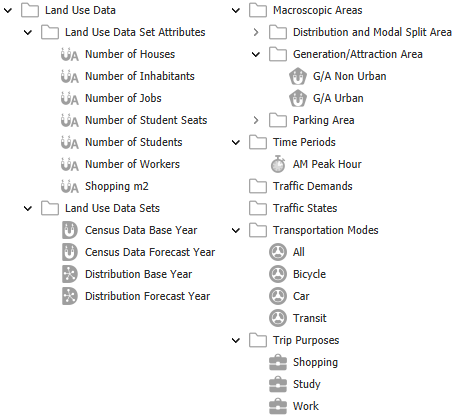
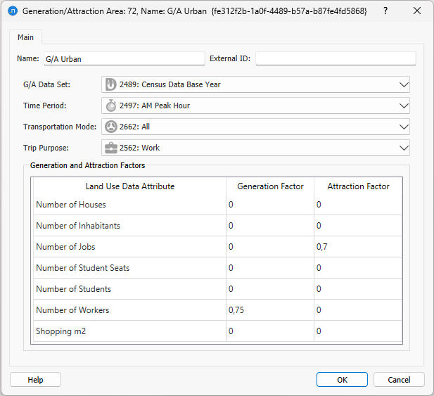
Double-click on any of the objects to see its parameters. For example, for the Generation/Attraction Area G/A Urban, the G/A factors are already defined for the base year, Time Period: AM Peak Hour and Transportation Mode: All.

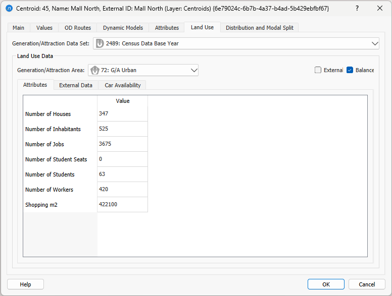
Now double-click on any centroid and click on the Land Use tab:

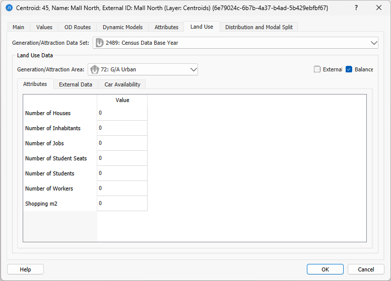
Some information is already present (the Data Set and Generation/Attraction Area are selected, the External Data checkbox and the Balance box are ticked where applicable) but the socioeconomic and land use values are all currently 0 and must be added in this exercise.

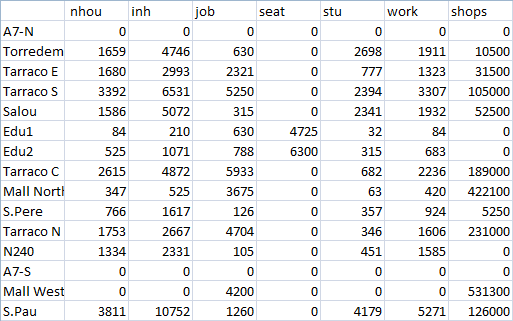
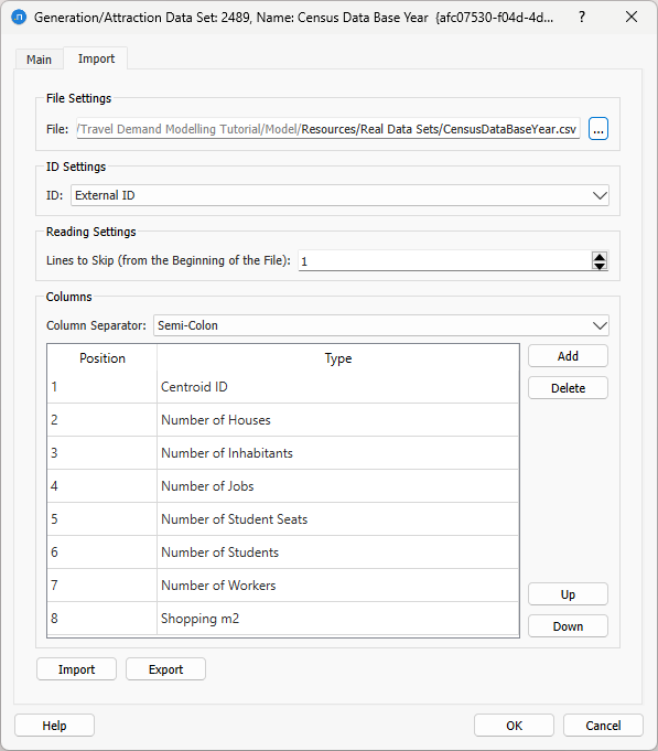
Together with the ANG file there is a Resources/Real Data Sets folder that contains a text file with the land use data for the data set named Census Data Base Year (CensusDataBaseYear.csv). Here is a screenshot of its contents:

To add the socioeconomic values:

1. Open the data set Census Data Base Year.

   Hint: Remember that you can find this object in the Project window under the folder Project > Demand Data > Land Use Data > Land Use Data Sets.

2. Click on the Import tab.

3. In File Settings, locate the data file CensusDataBaseYear.csv.
4. For ID Settings, select External ID.
5. In Lines to Skip, enter 1 (to skip the first, header, line of the CSV file).
6. For Column Separator, select Semi-Colon.
7. Click Add eight times to add eight new data rows.

8. Complete the rows as shown below (you can select the type of each column from the drop-down menu in each relevant cell).

   
   

9. Click Import to import the data from the CSV file.

10. Double-click the centroid again to verify that the data is now present:

    
    

1.2 Preparing and running the G/A Experiment

To add the G/A scenario and experiment:

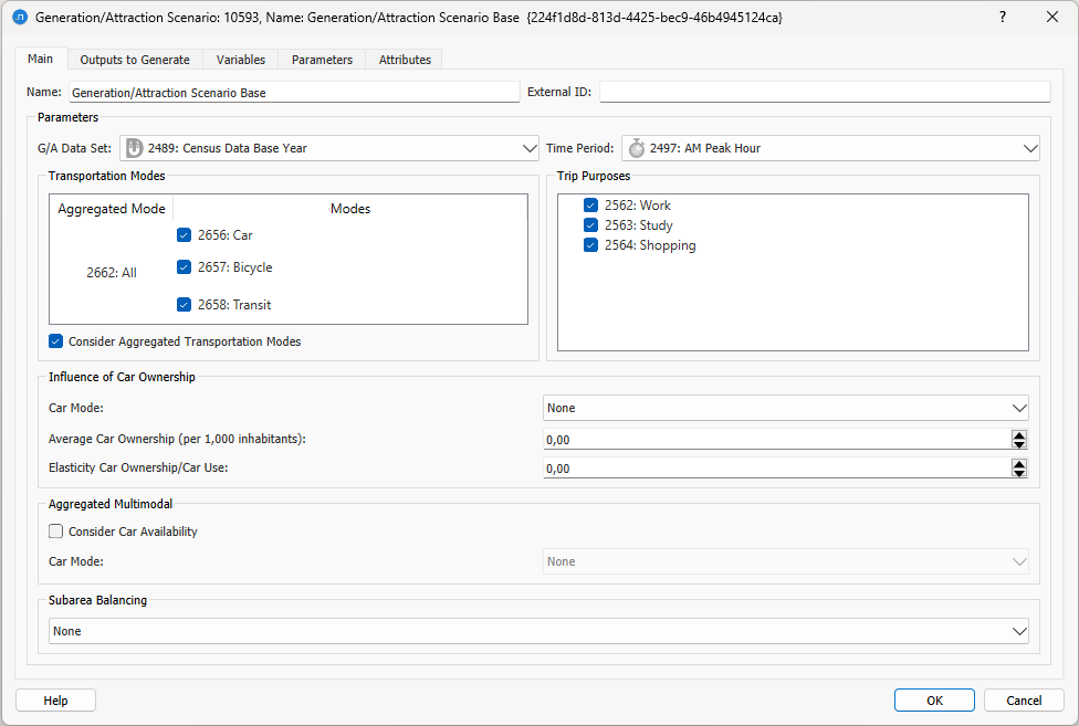
1. In the Project window, right-click Scenarios > New > Generation/Attraction Scenario.

2. Complete the parameters as shown below:

   
   

3. On the Outputs to Generate tab, tick Store in Database so that results can be retrieved later.

4. Click OK to save the scenario.
5. Right-click on the scenario and select New Experiment.

Now that we have a context which specifies the G/A data set we are working with, we can create a view mode and a view style to visualize some of the input data. If you need a reminder about creating view modes and style, see the earlier tutorial Viewing Microscopic Outputs.

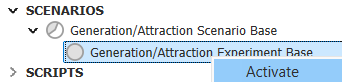
1. Activate either the G/A Scenario or Experiment through the corresponding context menu option.

   
   

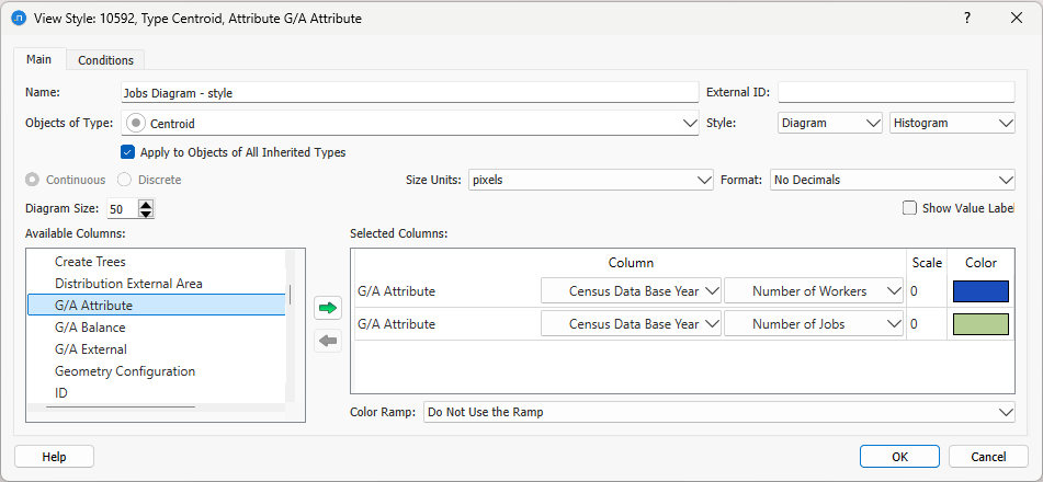
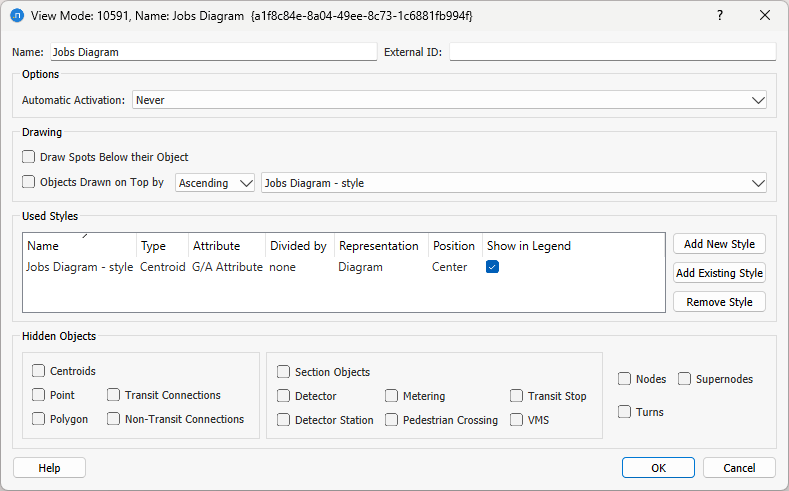
2. Create a view mode containing a view style and define them as illustrated in the next two screenshots:

   
   

   
   

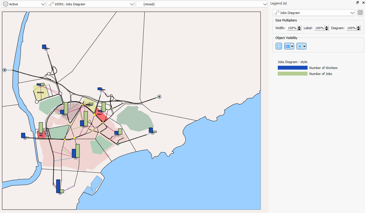
3. Apply the view mode to the view. You should see the histograms in the 2D view as shown below.

   
   

To run the G/A experiment:

1. Right-click on the experiment and select Run Generation/Attraction. The dialog, with summary results, is displayed when the experiment finishes.

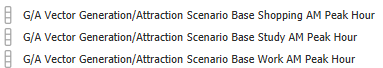
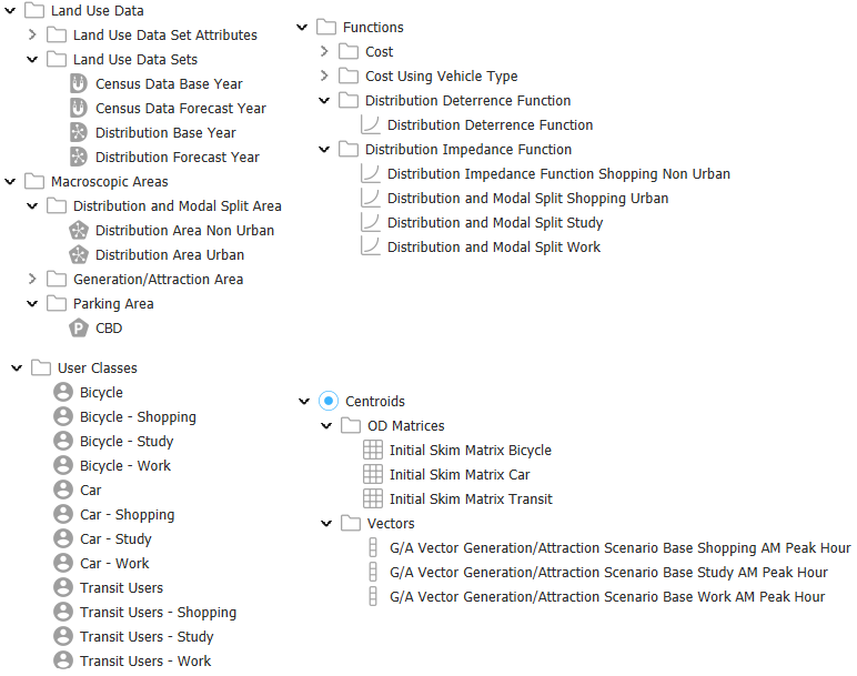
2. Click Generate Vectors to create the G/A vectors. These will appear in a new subfolder called Vectors inside the centroid configuration folder in the Project window. These vectors are the outputs of the process:

   
   

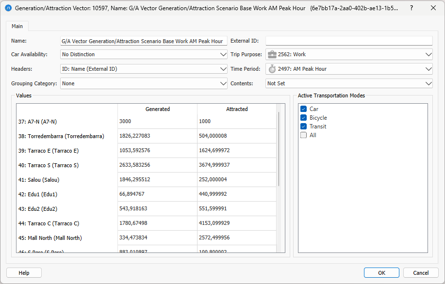
3. Double-click a vector to view its parameters:

   
   

Exercise 2. Running a Trip Distribution

Data inputs relevant to this exercise

• Centroids
• Distribution and modal split data sets
• Distribution and modal split area types
• Parking area types
• Time periods
• Transportation modes
• Trip purposes
• Skim matrices
• Distribution functions

In this exercise, we will look at the data needed for a trip distribution experiment, which will obtain a preliminary estimate of the travel demand.

Take a look at the data required for distribution: Distribution Sets, User Classes, Macroscopic Areas, Functions, G/A Vectors, and Skim Matrices containing costs.

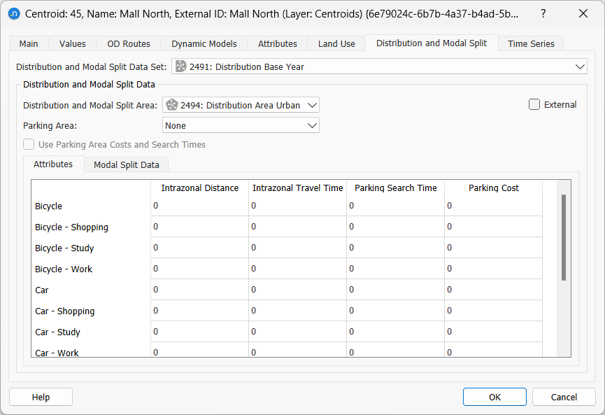
There is also centroid-specific data in the Distribution and Modal Split tab of a centroid dialog (see below).

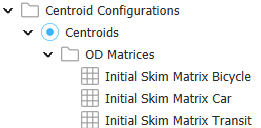
In order to run the distribution, we need to somehow quantify the accessibility between each OD pair. This information is extracted from the skim matrices, that contain the different costs (monetary, distance, travel time) that might be available. If a set of skim matrices is not available, at this point we would usually run some basic assignment experiments, with a dummy unit matrix traffic demand if no other estimate is available, to obtain preliminary estimates of the travel costs between each OD pair in each mode. In this exercise, however, we already have some initial skim matrices so we can omit the step of producing them, and directly use the available ones. You will find these skim matrices in the Project window here:

To set up a distribution scenario and experiment:

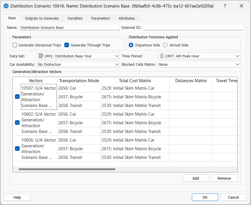
1. Select Scenarios > New > Distribution Scenario and define the parameters as follows:

   
   

2. Open the scenario editor and, in the Outputs to Generate tab, tick Distribution Results: Store.

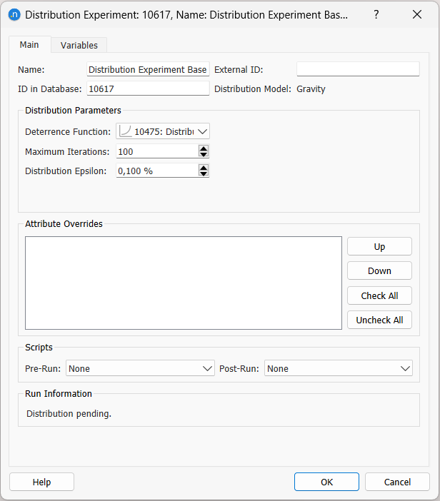
3. Right-click on the scenario and select New Experiment.

4. Select Distribution Model: Gravity Model and define the experiment parameters as follows:

   
   

Before proceeding with the distribution step, note that if you activate the distribution scenario or experiment, the context for the visualization of the previously calculated G/A vectors will be ready. Define a new view mode and view style to visualize one of these vectors in the network. In this case, for example, select Style: Diagram and Circles.

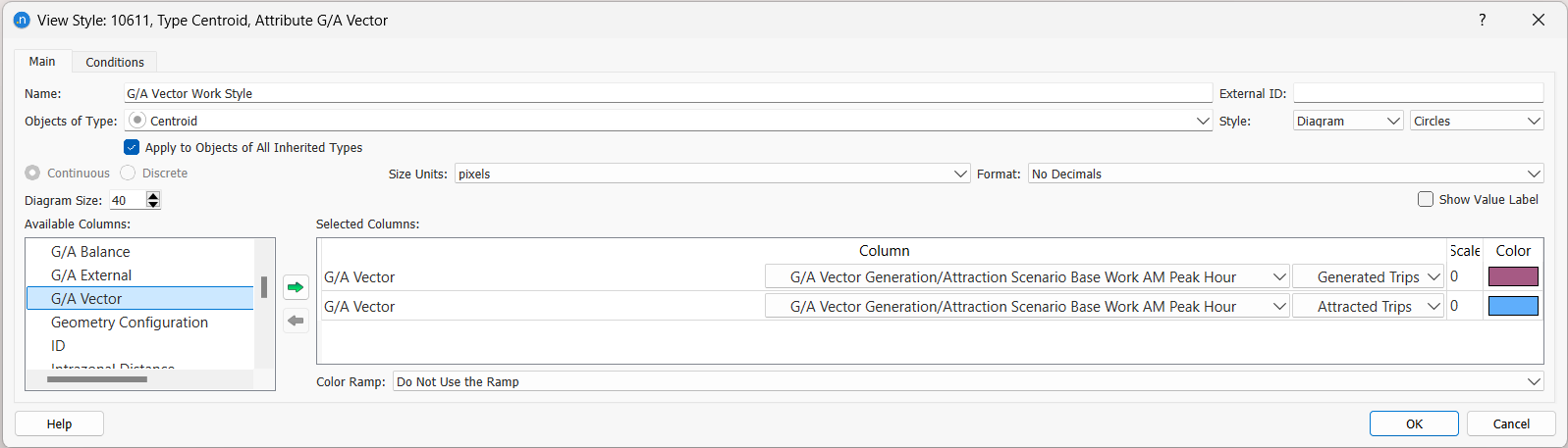
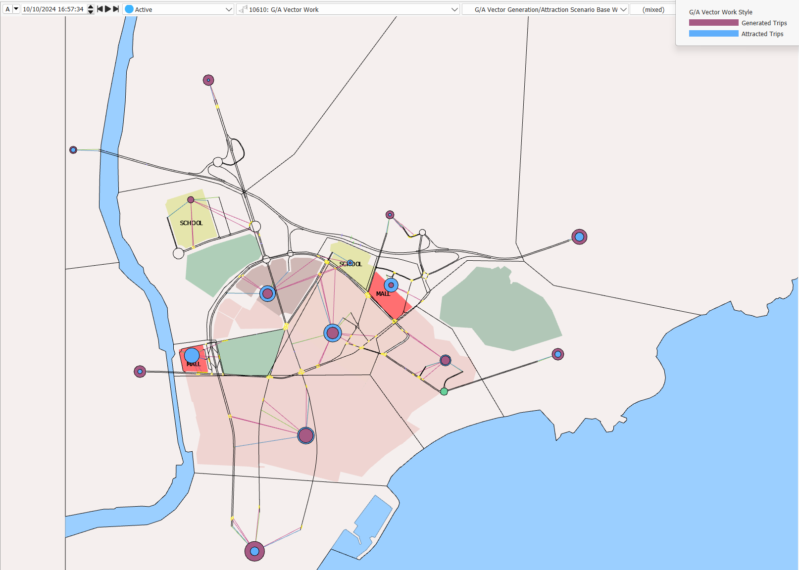
Apply the view mode to the view, as pictured below.

To run the G/A experiment:

1. Right-click on the experiment and select Run Distribution. The dialog, with summary results, is displayed when the experiment finishes.

   
   

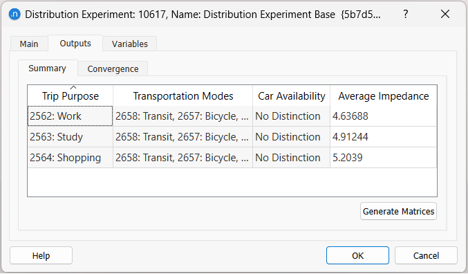
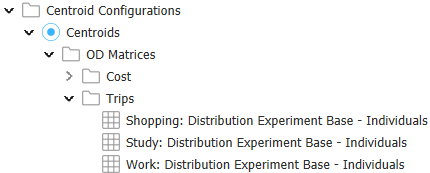
2. From this dialog, we can generate the OD matrices required for exercise 3. To do so, click Generate Matrices. The matrices are added to the Project window:

   
   

Exercise 3. Running a Modal Split

Data inputs relevant to this exercise

• Centroids
• Distribution and modal split data sets
• Distribution and modal split area types
• Time periods
• Parking area types
• Transportation modes
• Trip purposes
• User class occupancies
• Skim matrices
• Modal split functions

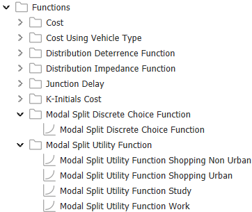
To run a modal split, we need to assign the modal split functions to the distribution area types. These functions are pictured below and you can find them in the Project window as usual.

To run a modal split:

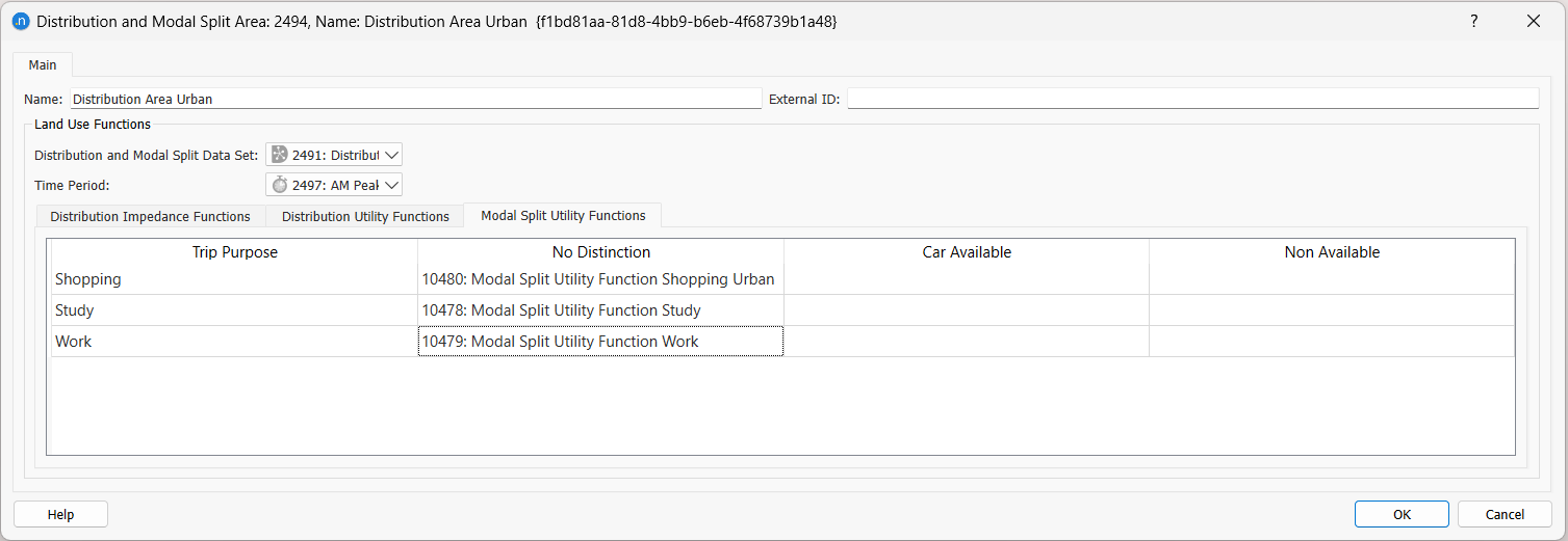
1. Open the distribution area named Distribution Area Urban and click on the Modal Split Utility Functions subtab. Alongside Trip Purpose Shopping, Study, and Work, set the modal split functions are selected as shown below in the No Distinction column. Do the same for Distribution Area Non Urban.

   
   

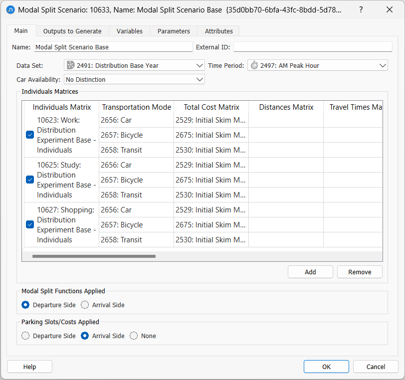
2. Select Scenarios > New > Modal Split Scenario and define the parameters as follows:

   
   3. In the Outputs to Generate tab, activate the option to Store Modal Split Results. 4. Right-click on the scenario and select New Experiment. 5. Double-click on the experiment and select the Discrete Choice function: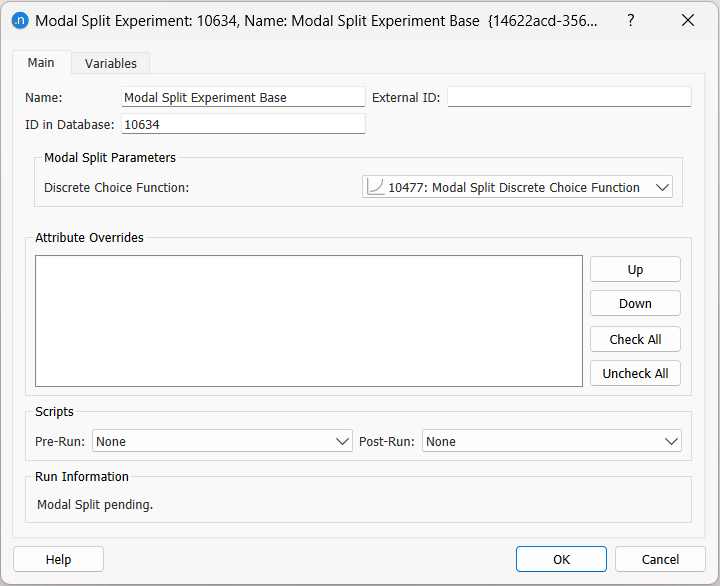

   
   

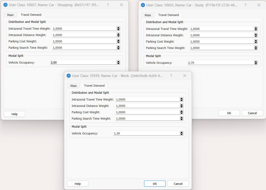
   For transit, the number of trips will be equivalent to the number of individuals (passengers). But the demand matrices for private transport should contain the number of trips in number of vehicles, not individuals. We will therefore add information to the user classes with vehicle type Car by providing the vehicle occupancy for each purpose. Bicycles don't need to be updated as the default is 1 individual - 1 trip.

3. Complete the Vehicle Occupancy parameter as follows: Car – Work - 1.3, Car – Study - 2.7, and Car – Shopping - 2.0:

   
   

4. We will assume that the City Business District (CBD) has a restricted number of parking spaces and we will provide this information for the CBD. Open the CBD area and add the number of Parking Slots as pictured below.

   
   

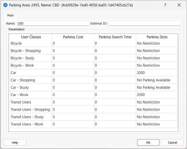
   We have specified 2000 spaces exclusively for cars that go to the CBD for work, plus 2000 for cars that go to the CBD for any purpose (work included). For Car - Shopping and Car - Study there is no specific number of slots available so we will set them to 'No Parking Available'. For the rest of non-car users, there is no parking restriction so we set them to 'No Restriction'. 8. Right-click on the experiment and select Run Modal Split. The Outputs tab will display the results on the Summary subtab.

   
   

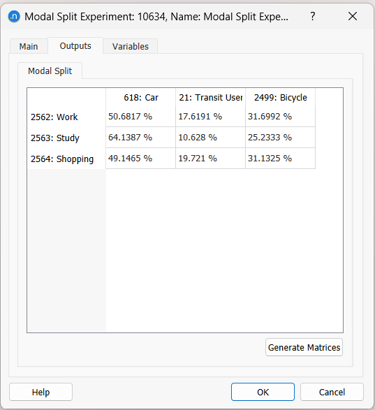
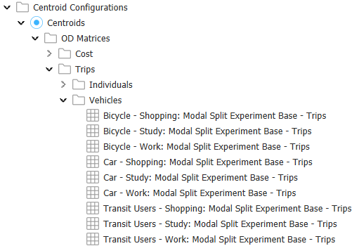
5. Click Generate Matrices to generate the OD matrices for static assignments. They will appear in the Projects window, as pictured below.

   
   

Exercise 4a. Running a Static Assignment

Data inputs relevant to this exercise

• Network
• Cost functions
• Private traffic demand matrices

In this exercise, we will assign the demand into the network. We have obtained nine trip matrices from the distribution and modal split experiments, one for each trip purpose and transportation mode.

Now we will create three traffic demand objects – one for each mode of transportation (bicycle, car, transit) – and add the three corresponding matrices to each demand. We need to do this because we are going to use a different assignment method for each transportation mode.

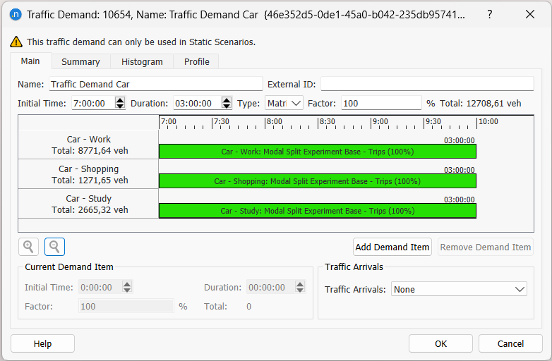
For example, the Traffic Demand Car will contain three OD matrices for the three user classes associated with vehicle type Car (the three different purposes).

To add the new traffic demands:

1. In the Project window, Right-click on Traffic Demands > New Traffic Demand.
2. Rename it Traffic Demand Car.
3. Open the new demand and click Add Demand Item.

4. Tick the three car-related demand item and click OK. Your demand should look like this:

   
   

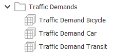
5. Repeat steps 1–4 but for bicycles and transit modes. You should have the following set of demands in the Traffic Demands folder.

   
   

Now we will add two scenarios and experiments in order to assign the car and bicycle demands.

1. Create and rename two static assignment scenarios.

2. For the car static assignment, select the Traffic Demand Car and set the Transit Plan.

   
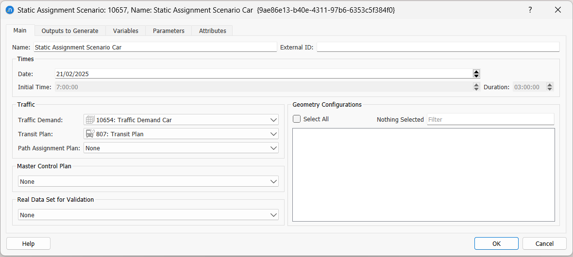   For the bicycle static assignment, select the Traffic Demand Bicycle. 4. In the Outputs to Generate tab, select the outputs to save: sections, centroid connectors and detectors, and turns and supernode trajectories. Activate the Path Assignment - Keep in Memory option as well.

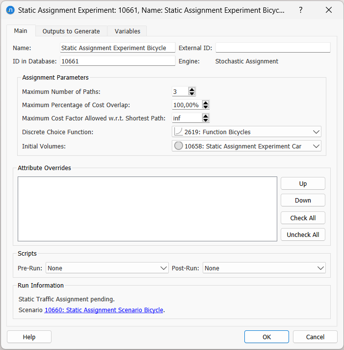
3. Create (and rename) an experiment within each scenario. For the car static assignment, select the Frank & Wolfe Assignment (equilibrium) method and for the bicycle static assignment experiment, select a Stochastic Assignment.

4. For the bicycle static assignment experiment, set its Maximum Number of Paths to 3. Set the Discrete Choice Function to Function Bicycles. Finally, set the pre-loads (Initial Volumes) in the network to use the Static Assignment Experiment Car results.

   
   

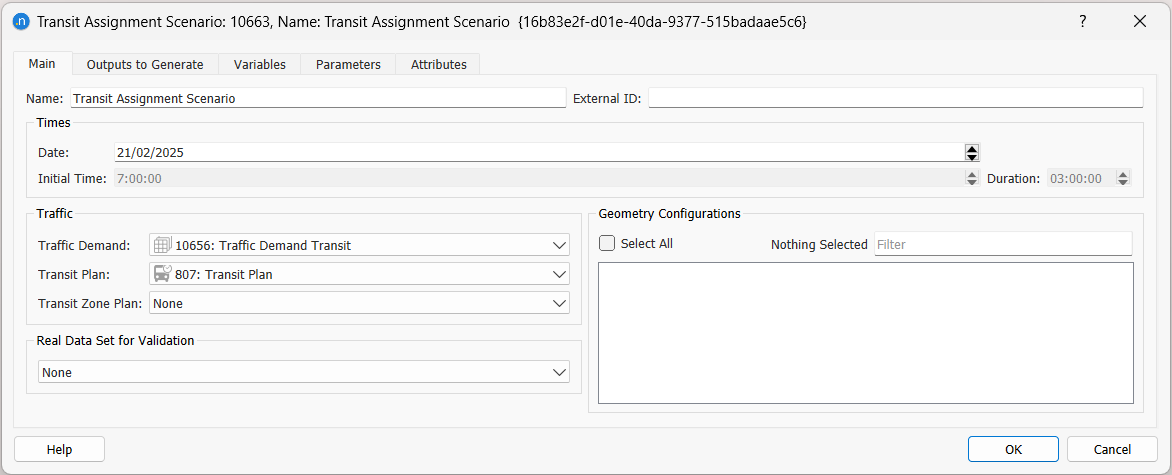
To add the transit assignment scenario and experiment:

1. Create the transit assignment scenario and complete the parameters as shown below, setting the traffic demand and transit plan:

   
   

2. In the Outputs to Generate tab, select the outputs to save: Sections and Transit Stops. Activate the Path Assignment - Keep in Memory option as well.

   
   

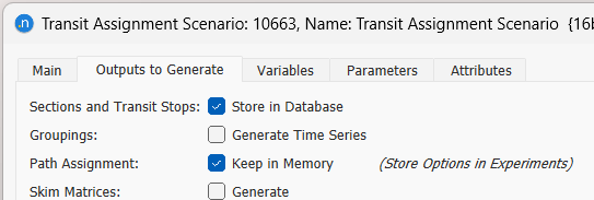
These will be stored in the database, with the ID of the experiment. 3. Right-click on the transit scenario and select New Experiment. 4. For the Assignment Method, select MSA Assignment.

Path assignment results are stored in APA files. A path assignment object contains the path where the file is located plus information about which experiment produced the data and which experiments are using them as inputs. In order to be the one in which the assignment stores the path assignment results, it has to be selected at the experiment level.

So we now need to create a Path Assignment for each one of the assignments. To create a path assignment:

1. Select Demand Data > New Path Assignment.

2. Open the new object to see its parameters.

   
   

3. Rename it Path Assignment Car.

4. Repeat steps 1–3 for Bicycle and Transit.

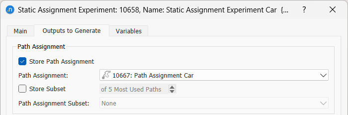
5. To store the path assignment data, open each one of the experiments, go to the Outputs to Generate tab, tick Store Path Assignment and select the correct Path Assignment object from the drop-down list.

   
   

Before running the car-related static assignment experiment, we can create three function components to retrieve some extra outputs from the assignment. These components will be travel time, distance and speed.

To add function components:

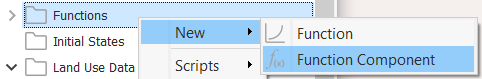
1. In the Project window, right-click Functions > New > Function Component.

   
   

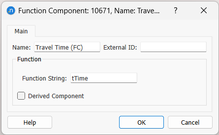
2. Define the travel time component as shown below.

   
   

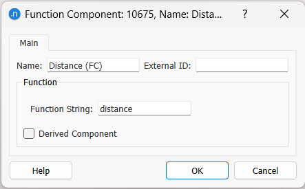
3. Repeat steps 1 and 2 for distance.

   
   

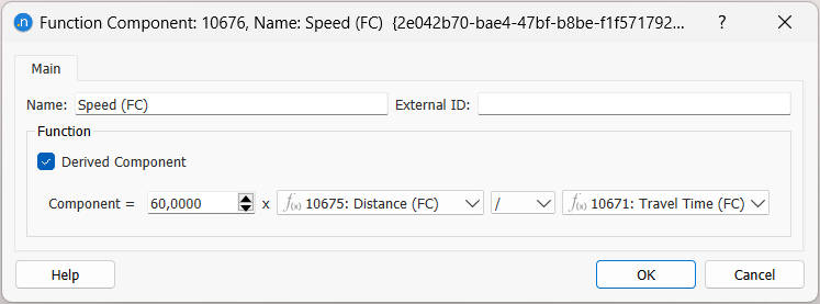
4. Repeat for speed, which is a derived component and requires to be defined as 60*distance/traveltime as, in this model, distance is measured in km and travel time in min:

   
   

To run the assignments:

1. Run the car static assignment first by right-clicking on the experiment and selecting Run Static Traffic Assignment.

   
   

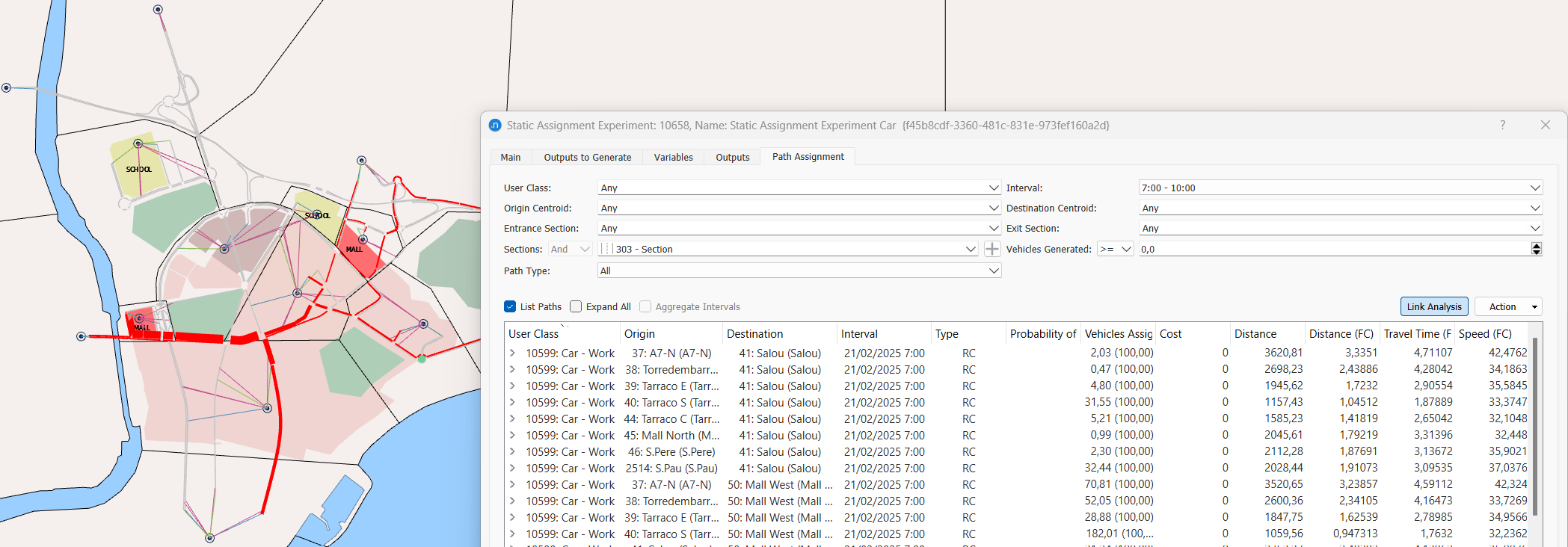
   The path-choice results are displayed on the Path Assignment tab of the static assignment experiment dialog. Take a look at the results and change the values of the parameters to explore the outputs, e.g. select a road section and click Link Analysis to see the paths of vehicles traversing that link.

   
   

2. Now run the bicycle static assignment experiment. This assignment takes into account the car assignment results as initial volume, and should be run second.

Exercise 4b. Running a Transit Assignment

Data inputs relevant to this exercise

• Network with centroid connections to and from transit stops
• Walking transfer costs
• Fare system
• Cost functions
• Passenger demand matrices

We have already set up the transit demand (in numbers of passengers) and the transit scenario and experiment. In order to proceed with the transit assignment:

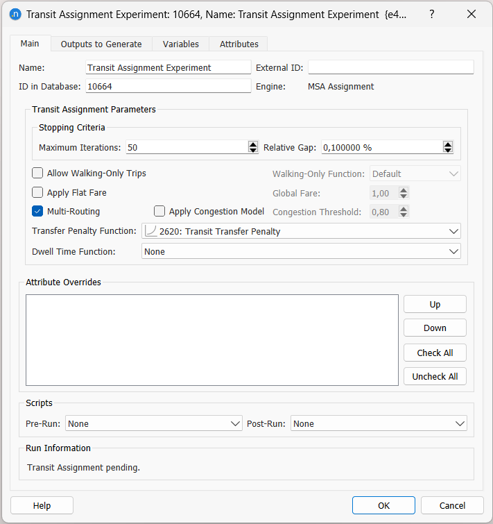
1. Complete the experiment's parameters by setting the transfer penalty function:

   
   

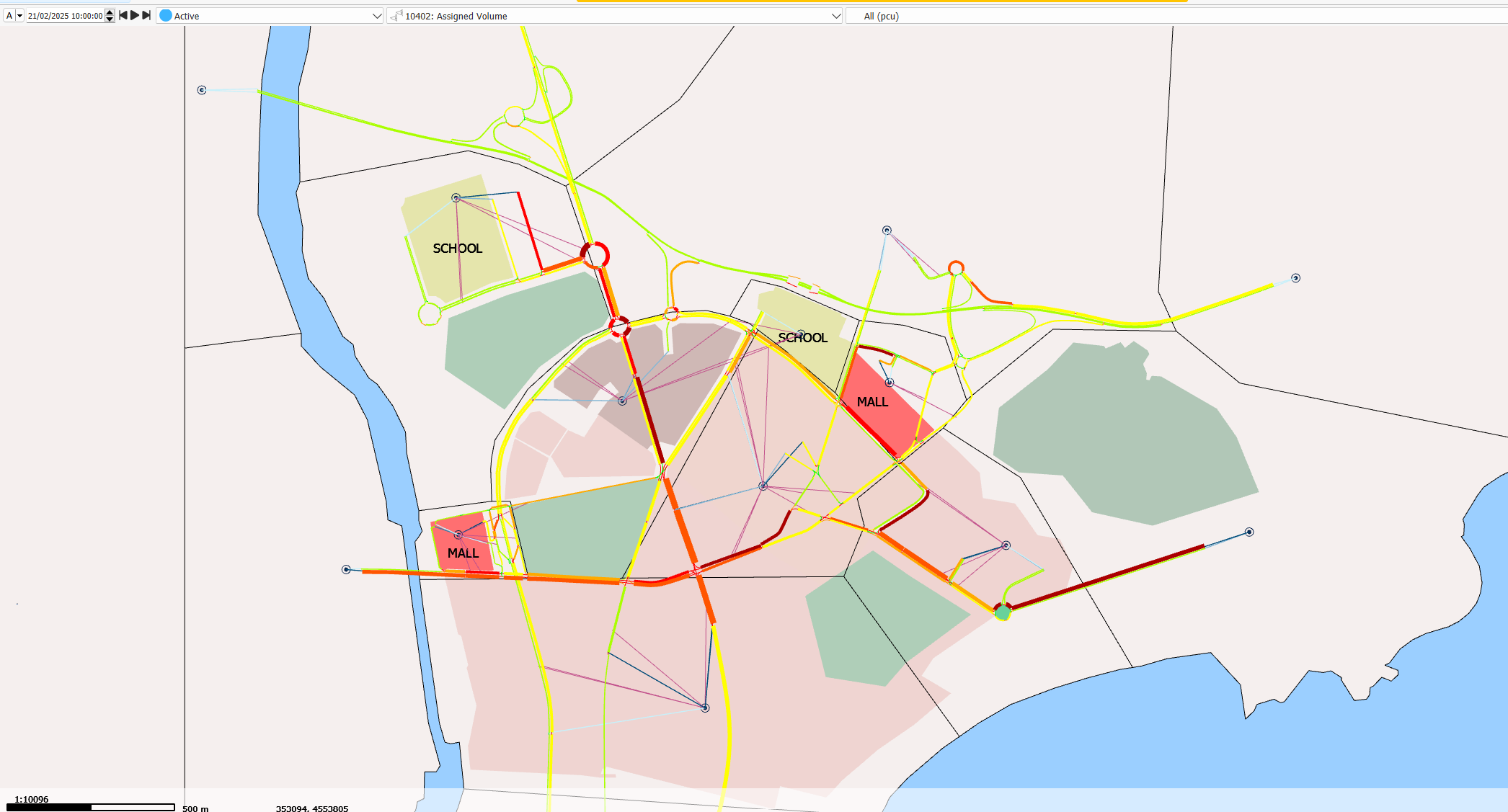
2. Run the experiment. The results are displayed on the Outputs tab and its array of subtabs:

   
   

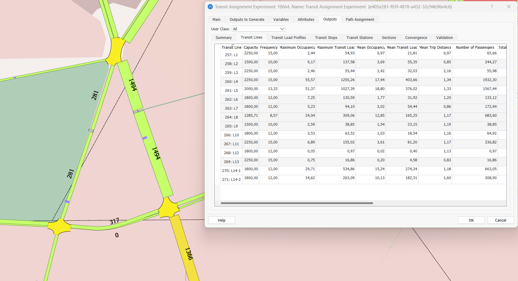
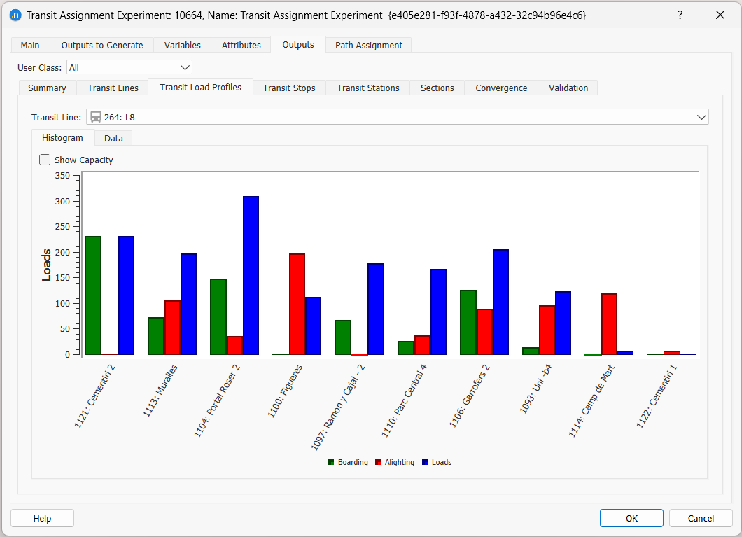
3. Check the transit assignment loads on the various subtabs.
   

Exercise 5. Running a Four-Step Model Experiment

In this exercise, we will bring the previous processes together by designing a four-step model experiment diagram that contains all the steps we have completed so far. Such a diagram is also useful for keeping track of the process that was developed to run the project.

To run a four-step model experiment:

1. Create a new four-step model scenario and add an experiment to it.

2. Open the experiment. You should see a blank grid as pictured below.

   
   

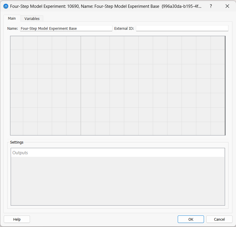
   In this space we can define the four-step model diagram, which consists of interconnected boxes that represent the experiments and outputs we have generated so far in this tutorial.

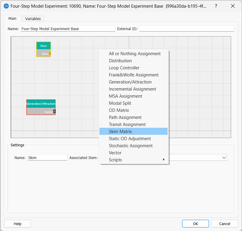
3. To add boxes, right-click on the grid and select the appropriate category (e.g. Generation/Attraction, Distribution, Modal Split, Skim Matrix, etc.).

   
   

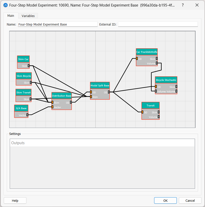
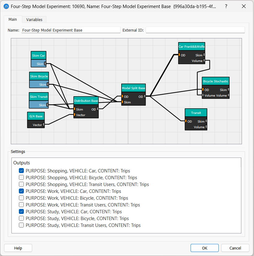
4. Add all the boxes related to the processes we have run so far and link the boxes together by dragging links with the mouse from one box to another. Aim to produce the result pictured below.

   
   

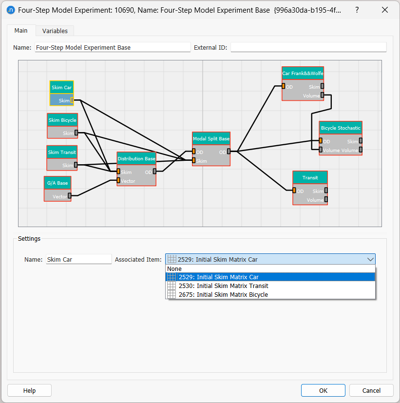
5. Complete the Settings information for each box and arrow. Start by relating each box to each object or experiment and renaming the box correspondingly. The first screenshot below shows how to link the Skim Car box with its Associated Item from the drop-down list.

   
   

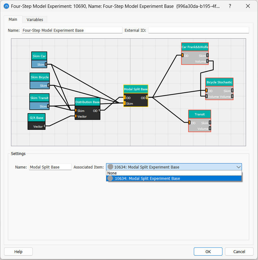
   The next screenshot shows how to link the Modal Split process box to the correct modal split experiment.

   
   

   Not only the boxes need to be correctly associated with the corresponding objects and experiments, but also the links content must be set up, so that only the selected outputs from one process become inputs for the next process. Click on each link and review its contents. For example, the next image shows the right contents to pass through from Modal Split step to the Car Static Assignment, which are the three car matrices, one for each trip purpose.

   
   

6. Run the experiment from the Project window by right-clicking on it and selecting Run Four-Step Model.

You can further define the boxes in the diagram, add intermediate scripts or add a loop box to make the process iterative until a certain stopping criteria is met.