Meso Traffic Modeling

The main difference between the mesoscopic and microscopic approach is the use of discrete events to simulate vehicle movements through the network rather than the simulation of discrete time steps. With this exception, most of the modules and concepts in Aimsun Next are shared between meso and microscopic simulation. For example, the vehicle entrance process, traffic demand data, network geometry, vehicle data, and control plan are common to both modes.

Note about licenses: Mesoscopic simulation is available in Aimsun Next Advanced, or Expert Edition annual-subscriptions.

Vehicle Entrance Process

The traffic generation process (arrivals) determines the headway times between vehicle arrivals. These headways are used to generate the vehicles that will enter using dynamic network loading. Vehicles enter into the network via origin centroids, where an origin centroid can be connected either to a section or to a node. The network structure for both situations is depicted in the screenshot below.

In both cases, vehicles enter the real network through virtual turns when the node server considers that there is enough space in the network for the vehicle to get in (and queue in a virtual section upstream if there is no space to enter).

Modeling Vehicle Movement

Vehicle movement is divided into two models:

• Modeling vehicle movement in sections
  • Car-following
  • Lane-changing
• Modeling vehicle movement in nodes (Node Model)
  • Modeling vehicle movement in turns
  • Modeling vehicle movement from sections to turns
    • Apply gap-acceptance model
    • Apply lane-selection model

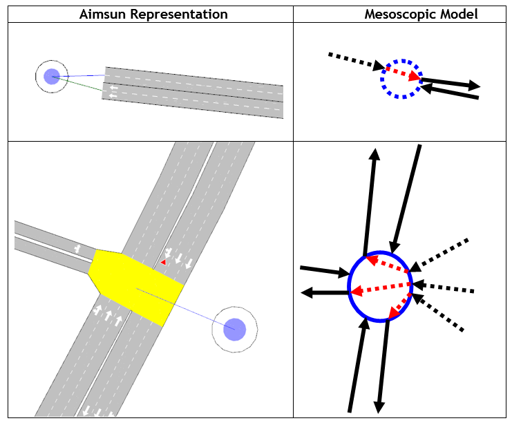
In Aimsun Next, the main network elements are sections and turns that connect two sections (and nodes, which are containers of turns). In the mesoscopic network representation, nodes are interpreted as mesoscopic nodes.

In a mesoscopic simulation, vehicles are assumed to move through sections and turns, so sections and turns become vehicle containers. A direct consequence of this is that all nodes are considered to be non-yellow boxes. The SectionCapacity, in terms of the number of vehicles that can be contained at any time in a section, is calculated according to this formula:

  SectionCapacity = JamDensity * Length * NumberLanes

where

• JamDensity is the Jam Density parameter defined in road sections
• Length is the section length, considering 3D coordinates
• NumberLanes is the total number of lanes in a section, considering on- and off-ramps

The turn capacity TurnCapacity is calculated in a similar way:

  TurnCapacity = JamDensity * Length * NumberLanes

• JamDensity is the Jam Density parameter of the origin section
• Length is the turn length, considering 3D coordinates
• NumberLanes is the total number of destination lanes

Car-following and lane-changing models are applied to calculate the section travel time. This is the earliest time a vehicle can reach the end of the section, taking into account the current status of the section (number of vehicles in the section). Modeling of vehicle movements on sections in the mesoscopic simulator is based on the work of Mahut (1999a, 1999b, 2001).

The expected maximum capacity per lane (veh/h), or max throughput flow, \(Q_{max}\), can be calculated with the following formula:

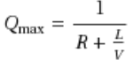
where - R is the global reaction time (set in the experiment) multiplied by the section reaction time factor - L is 1/JamDensity - V is the speed limit

Reaction Time Factor

The reaction time factor can be set at both section and turn levels. The section reaction time factor is used in the following situations:

• Ramp Meters, when changing from red to green.
• Lane selection model to select the departure lane.
• Car-following model to calculate the intermediate section entrance times in the particular case of sections that are cut internally for the model calculations, for example when there are on/off-ramps or incidents.
• In the car-following model the reaction time of the vehicle leader is also used to calculate a minimum headway with this leader. In this calculation the section reaction time factor is also applied.
• Queue stats, in order to calculate the queue statistics the vehicle reaction time is used to calculate the waiting time in queue. In this calculation the section reaction time factor is applied. See in Mesoscopic Queue Length how the vehicles are considered to be in queue.

The turn reaction time factor is used in the following situations:

• Traffic lights, when changing from red to green.
• Car-following – when the vehicle is in the turn, the turn reaction time factor is used to calculate the node-exit times of the other turns that have spatial conflict with the turn, and it's also used to calculate the entrance time when the vehicle is about to enter the next section.

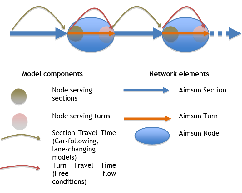
Node Model

The Aimsun Next mesoscopic simulator is based on a node model that moves vehicles from one section to the next section of their path. This model contains four classes of occurrences that are calculated in all nodes:

• Serving sections. This calculates the next vehicle to enter the node (leaving the queue server at the end of the section). This is done by applying the yield model if required, and by using the section-exit times calculated by the car-following and lane-changing models. Once a vehicle has been identified as the next vehicle to enter the node (exit section), the next vehicle position in queue is updated.

  By doing this we ensure that all delays produced by downstream congestion are propagated to upstream vehicles. The mesoscopic simulation is event-based, so there is an event related to this action or network-state change. The event concerns the next vehicle to enter the node from any of its input sections. This event is called a "node event from section".

• Node event from a section. When processing vehicles' exit from a section, the actions are:

  • Calculate vehicle-turn travel time. This calculation is done using the assumption that lane changes are not allowed under any circumstance inside nodes. Therefore, this travel time is always considered in free-flow conditions.
  • Apply the lane-selection model to determine the entrance and exit lanes during the next section movement. This uses the valid target lanes model.

• Serving turns. This server calculates the next vehicle to leave the node (entering the next section). To get this vehicle, the exit turn time and the conditions of the vehicle's downstream section are taken into account. Once a vehicle has been selected, a new event called "node event from turn" is scheduled.

• Node event from a turn. Processing vehicles' exit from a node implies the following:

  • Move the previously identified vehicle to its next downstream section and queue this vehicle at its departure lane.
  • Apply the car-following and the lane-changing model to calculate the vehicle travel time, including the delay due to lane changing, and calculate the earliest time that this vehicle will reach the end of the section.

Gap-Acceptance model: Non-priority behavior

In a mesoscopic simulation the yield and stop are simulated using the same behavior model. It is important to note that in the mesoscopic simulation, vehicles do not use the acceleration and deceleration components in their car-following model. Vehicles in a mesoscopic simulation are considered to always travel at their target speed. This restriction is important in all situations where acceleration and deceleration plays an important role in the calculation of vehicles' travel time, in particular in all situations with a stop sign. It is therefore difficult to compare two simulations using mesoscopic and microscopic behavior models with stop signs.

The yield model is used to model yield behaviors. In particular, the model is used when resolving node events in order to decide which of two vehicles in a conflict movement have priority. The following screenshots show some examples of conflict movements.

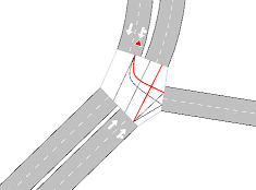
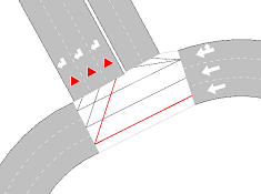
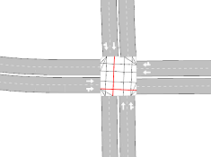
The yield model is applied only in the first and second examples in the previous screenshots. In the third example, vehicles do not have any yield or stop signs, so the model is not applied and the first-in, first out (FIFO) rule is applied by using the corresponding vehicle demand times. Note that the vehicle demand time is the time at which the vehicle is ready to move to the next turn.

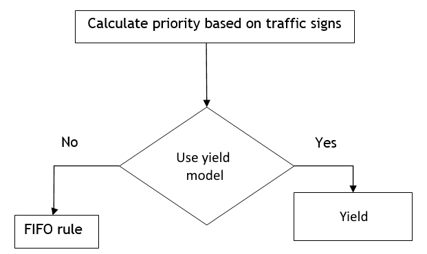
The general model is as illustrated below.

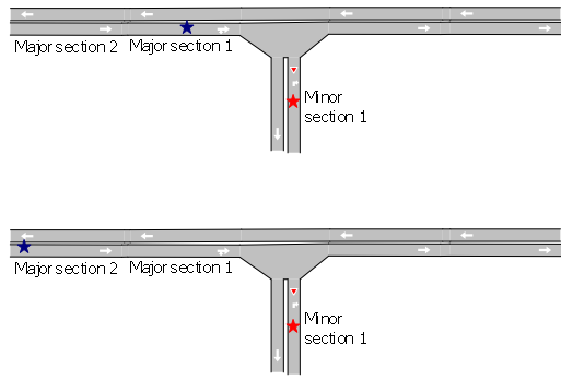
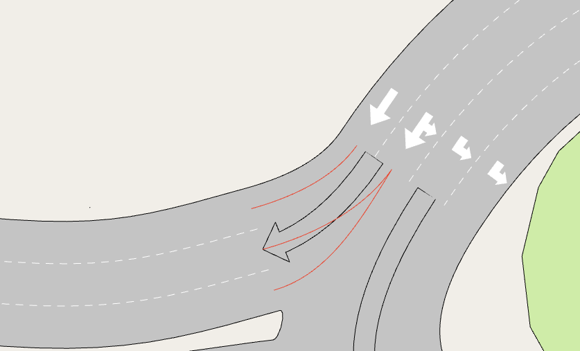
The yield model used in the mesoscopic approach is a simplification of the yield model used by the microscopic simulator. The model takes into account the demand times of vehicles that are approaching the conflict movement. Demand times are used to calculate the gap required for a vehicle with a yield restriction to enter into the node. In the next screenshot, the red vehicle has to yield to the blue vehicle.

Let \(TD_R\) be the demand time of the red vehicle. This is the current time estimation for the red vehicle to enter into the node. Let \(TD_B\) be the demand time of the blue vehicle. This is the current time estimation to enter into the node with the conflict movement.

If there is no vehicle in the immediate input sections to the conflict node then the model looks for vehicles upstream until a maximum distance is reached. In the second screenshot below, Major section 1 is empty, so the model looks at its upstream section, which in this case is Major section 2. The value of \(TD_B\) now takes into account the demand time of the blue section in Major section 2 and then calculates the travel time of Major section 1, in free flow, to calculate the \(TD_B\). Only vehicles in the main stream with trajectories that are in conflict with the red vehicle are considered.

In this example, if the blue vehicle turns right instead of going straight ahead the red vehicle has no need to yield. The distance that the model looks upstream can be set in the road type or turn editor and is called Visibility along main stream: see the Road Type Editor or Turn Editor.

Once \(TD_R\) and \(TD_B\) have been calculated, the gap is (\(TD_B\) - \(TD_R\)). This is used to decide whether the red vehicle needs to yield or not. The waiting time of the red vehicle is used to calculate the maximum gap using the function in the next screenshot. This shows how the required gap changes as a function of a vehicle's waiting time. If the gap is in the blue shaded area then the red vehicle can pass through the node; otherwise it has to stop and cannot enter the node.

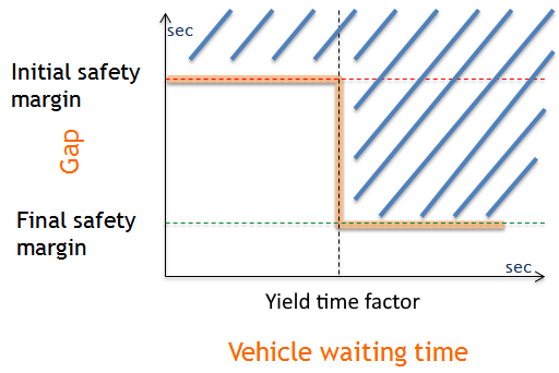
The initial safety margin, final safety margin and yield time factor can be changed in the road type or in the turn parameters. Initially, the vehicle has to wait in the minor section until it has a gap greater than the initial safety margin. Once it has waited until the vehicle's maximum yield time multiplied by the yield time factor, the minimum gap required to make the movement is reduced to the final safety margin.

Lane-Selection Model

This model is used to calculate the section entrance and exit lanes. As described in the node model, these calculations are made during the treatment of the "Node Event from Sections" event which occurs before the vehicle enters the turn.

Section entrance lane selection

Each turn has a set of turn connections that describe, within the valid lanes of the turn, from which lane from the origin section you can reach each lane in the destination section.

The mesoscopic simulator distributes the vehicles from a turn among the different entrance lanes in the next section trying to increase the headway between vehicles in each entrance lane. That means, in the following example, that the vehicles coming from the rightmost lane and turning right will stay in the rightmost lane, while the ones turning right but coming from the second rightmost lane will alternate (in free-flow conditions) between the central and leftmost lane to enter the destination section.

The next section status will also be considered. For each turn there is a queue for each turn destination lane (section entrance lane). The capacity of these queues is the jam density of the origin section multiplied by the turn length. When having more than one option, if any of the available options is full, the vehicles will distribute among the others.

In some situations, like in urban networks where there are short sections, or on freeways where weaving sections are relatively short, vehicles will take downstream turn movements into account in their lane-selection decision. Thus, the look-ahead will also be taken into account in this selection, both for entrance and exit lane selection. For the next section entrance and exit lane under the look-ahead effect, the valid target lanes model implemented in the mesoscopic simulator uses the same approach as in the microscopic simulation.

Section exit lane selection

The exit lane from a section is, as well as the entrance lane, calculated when entering the previous turn.

When there are multiple possible lanes, a penalty is calculated for each lane. The penalty function is based on the number of lane changes needed to reach the target lane and the densities observed on each lane of the section. There are two optional penalties that can be set for each section:

• Penalize shared lanes. When this option is ticked, a penalty is added for those lanes that belong to different turns.

• Take into account fast/slow lanes. This option favors fast vehicle types using fast lanes (leftmost in a right-hand rule of the road model) and slow vehicle types using slow lanes.

Both penalties are the same as those that are used to penalize the number of lane changes.

Once a penalty is calculated for each lane, the lane with the minimum penalty is selected. If there are multiple lanes with the same minimum penalty, the lane is selected at random.

Mesoscopic Simulation: Random Seeds

Random seeds usage is common for both micro and mesoscopic network loading, please refer to the Microscopic Randon Seeds section for the description and usage of the different random seeds, general and specific.

Since the different random seeds are available in both meso and micro, they can also be applied in hybrid meso-micro.

Mesoscopic On-Ramps and Off-Ramps

To model on-ramps and off-ramps, the mesoscopic simulation cuts the section with the ramp into different segments. For example, the following road section has two internal segments; the first segment has three lanes and a length of 100 meters and the second segment has two lanes and is 300 meters long.

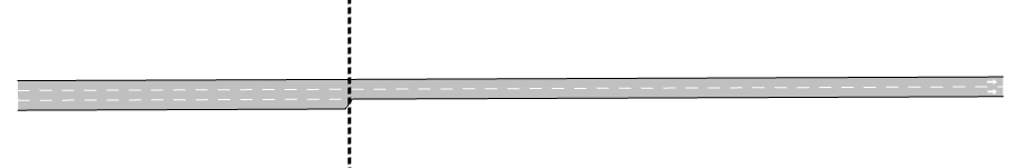
Internally, this is translated as two sections with a different number of lanes as shown below. The closest lane to the ramp will have 2 connections - to/from the direct lane connection and to/from the ramp.

It's very similar but not completely the same as the following geometry:

Here, instead of an on-ramp being part of the section, the on-ramp is implemented as two different sections connected with a node and a turn (with some length). By definition, all turns have a minimum capacity of one vehicle, so in this last case vehicles will move from the section upstream to the turn, and then from the turn to the next section downstream. In the case of the ramps, however, there will be direct connections between the lanes in the segment upstream and the segment downstream, but no turn and node entities. In general, it is more convenient to model on-ramps by coding them as in the first example.

For the specific case of off-ramps, the lane in the upstream that is closest to the ramp in the segment downstream will have 2 connections and will spread the traffic uniformly among the target lanes (taking into account the look-ahead).

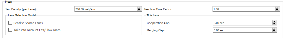
For the specific case of on-ramps, in addition, there are two parameters that you can use to calibrate its behavior: Cooperation Gap and Merging Gap.

• Cooperation Gap: It is the amount of time (in seconds) that the mainline vehicles will force to have as headway whenever side-lane (on-ramp) merging vehicles are present. This is to facilitate the incorporation of traffic. The only vehicle that will be delayed is the vehicle on the first mainline lane adjacent to the ramp.

• Merging Gap: It is the minimum gap that vehicles in the side lane (on-ramp) look for in order to merge into the mainline.

Mesoscopic Queue Length

The queue length in a mesoscopic model is the average number of vehicles that have a delay, weighted with the amount of delay each vehicle experiences. In a mesoscopic model, a vehicle either moves at its desired speed, or is stopped at the end of a section. The vehicle experiences the accrued delay at the end of section. This includes the delay from other vehicles waiting in front, signals and from the conflicts of opposing turns. So, when a vehicle traveling through a section or turn, the time that a vehicle stays in the queue server is defined as the time spent queueing.

Mesoscopic Initial State

A mesoscopic initial state is different from the microscopic initial state. The microscopic initial state holds a set of vehicles and these vehicles are inserted into the network. In a mesoscopic model, the initial state stores the network status, vehicle definitions and positions and the internal variables used in the mesoscopic calculations. The initial state is then only valid if the network is exactly the same. Any change in the supply or any change in the transit definition can invalidate the initial state.