Static OD Departure Adjustment
Departure Adjustment
The static OD departure adjustment method has been developed as an improvement to the original matrix slicing in which the dynamic traffic demand is obtained by slicing the simulation time in a number of periods and then each slice is adjusted independently.
This method works well if travel times between origin and destination are short with respect to the period, but shows a bias in departure time for longer trips because the travel time aspect is neglected. The static departure adjustment solves this problem by taking into account the travel time obtained from the static assignment in calculating the dynamic traffic demand.
Problem definition
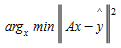
The objective is to find a dynamic demand x that minimizes the sum of the squared distances between the observed counts yˆ and simulated counts y, with the assignment matrix A and y = Ax this can be written as:
In order to construct the assignment matrix that maps the dynamic demand to the observed counts, the following assumptions are made:
- Link travel times are constant over the simulation period.
- Path choice is constant over the simulation period.
- The demand is uniformly generated during each time slice.
The following definitions are used:
- x~0~ is a vector containing trips for each origin a to destination b: x~0ab~.
- I are the intervals, which can be departure or detection intervals, depending on what they reference.
- D is the time slice (interval) duration.
- C is the set of links with counts.
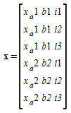
- x is a vector containing trip proportions for each origin a to destination b for each departure interval d: x~abd~.
- yˆ is a vector containing observed counts for each link c for each detection interval e: yˆ~ce~
- y is a vector containing simulated volumes for each link c for each detection interval e: y~ce~
- K~ab~ is the set of paths used from a to b.
- t~kc~ is the travel time to link c using path k.
- p~k~ is the proportion of usage for path k
Each cell of the matrix A can be constructed with:


where:

Based on the calculation of the fraction of demand of an OD pair departing at interval d that passes through a detection point at interval e.
Example:

In this example the time to travel from origin a to link c by path p is 0.75D so 25% of the demand generated in interval 1 passes link c in interval 1 and 75% of the demand generated at interval 1 passes link c in interval 2.
Conservation of demand
The objective of the static departure adjustment is to calculate the dynamic demand from a static demand, therefore it is desirable that the OD trips are conserved and only distributed in time. To obtain this, the following equations are added to the original problem definition:

Meaning that the fractions for all intervals for a particular OD pair must sum to 1, so that the OD flow is preserved.
Result
The equations for the assignment matrix and the conservation of demand are a linear system of equations that can be readily solved in a least square sense with standard solutions methods such as gradient descent methods. multiplying the original demand with the calculated fractions x gives the dynamic demand.
Example
Consider the following example network to illustrate the process.
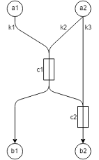
There are two OD pairs; a1-b1 using path k1 and a2-b2 using 33% path k2 and 67% path k3. Path k1 passes through detection point c1, path k2 passes through detection points c1 and c2, and path k3 passes through detection point c2.
Travel times are:
- from a1 to c1 using path k1 : 5 minutes
- from a2 to c1 using path k2 : 5 minutes
- from a2 to c2 using path k2 : 10 minutes
- from a2 to c2 using path k3 : 5 minutes.
The simulation time is 45 minutes divided in three 15 minutes intervals (i1, i2, i3). During these 45 minutes, 1000 vehicles go from a1 to b1 and 1200 vehicles go from a2 to b2. Finally, observed counts for the two detectors are:
- c1: ( 180, 520, 530 )
- c2: ( 130, 500, 450 )
Then:
and
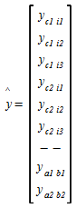
In which y~a1b1~ and y~a2b2~ are equal to one reflecting that demand should be conserved. Now we can calculate the matrix A by calculating the assignment matrix and adding the equations for demand conservation:
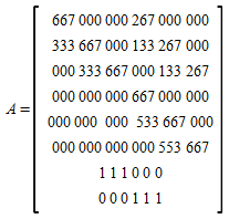
Observed data + demand conservation equations give:

The solution is then given by:
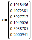
From which the dynamic OD trips can be obtained easily by multiplying the factors with the original OD volume giving:
- a1-b1: ( 192, 407, 393 )
- a2-b2: ( 234, 712, 240 )