Integrating Macro, Meso, Micro, and Hybrid Simulations¶

Note about licenses: These exercises require a license for Aimsun Next Advanced or Aimsun Next Expert Edition.

Exercise 1. Using a Static Assignment to Verify Real and Simulated data
Exercise 2. Defining a Subnetwork Study Area and Running a Static Traversal
Exercise 3. Checking Detector Coverage
Exercise 4. Extending the OD Matrices Based on Traffic Measurements
Exercise 5. Adjusting the Subnetwork OD Matrices
Exercise 6. Creating a Profiled Demand with a Static OD Departure Adjustment
Exercise 7. Running a Dynamic User Equilibrium (DUE) Experiment, Loading Static Paths
Exercise 8. Running a Microscopic Stochastic Route Choice (SRC) Scenario, Loading DUE Dynamic Paths
Exercise 9. Running a Meso-micro Hybrid SRC Scenario, Loading Dynamic Paths
Exercise 10. Running a Macro-meso Hybrid Simulation

Introduction¶

In these exercises we will step through the project workflow that integrates macroscopic, mesoscopic, microscopic, hybrid macro-meso, and meso-micro simulators in Aimsun Next. We will see how a modeler can combine different levels of network loading in the same model file.

Some of the longer exercises are split into two or more separate procedures.

In Exercise 1 we will assign the original OD matrices to the traffic demand. Then we will run a static assignment scenario and review the output, comparing it to observed real-world data loaded as a real data set.

In Exercise 2 we will create a subnetwork of our study area and run a static traversal. This will create the OD matrices for the subnetwork. The traversal will be based on the static assignment results generated in Exercise 1. We will then run a static assignment for the subnetwork and review the traversal outputs.

In Exercise 3 we will check to see whether the study area is adequately monitored by detectors.

In Exercise 4 we will use traffic counts to calculate the weight factor required to extend the hourly OD matrices from 08:00–09:00 to 06:00–10:00.

In Exercise 5 we will run a static OD adjustment scenario to refine the OD matrices to align them with the observed data.

In Exercise 6 we will run a static OD departure adjustment to create a profiled demand from a static demand using a static OD departure adjustment.

In Exercise 7 we will run a dynamic user equilibrium (DUE) experiment to derive a new set of paths, this time based on a DUE simulation.

In Exercises 8 and 9 we will compare the results of a micro SRC simulation using dynamic paths (paths resulting from the previous DUE iteration) with a hybrid meso-micro SRC using the same paths. We are looking for similar results in terms of flow, delay, time, and speed.

In Exercise 10 we will run a hybrid simulation using macroscopic and mesoscopic network loading in a single experiment.

Exercise 1. Using a Static Assignment to Verify Real and Simulated Data¶

In this exercise we will use the macroscopic simulator to assign the number of trips to both OD matrices (vehicle types: car and truck) throughout the traffic network. The resulting assigned volumes will be compared to the observed data after creating a real data set object as a sense check to verify that the data has been imported correctly.

Before we begin, open the strategic model of Bilbao (integration_ini.ang), which can be found in [Aimsun_Next_Installation_Folder]/docs/tutorials/7_Integration].

1.1 Creating a real data set object¶

First we need to create a real data set object to retrieve traffic-measured detector data to use for validating our eventual results.

Select File > Open and locate integration_ini.ang.
Click Open.
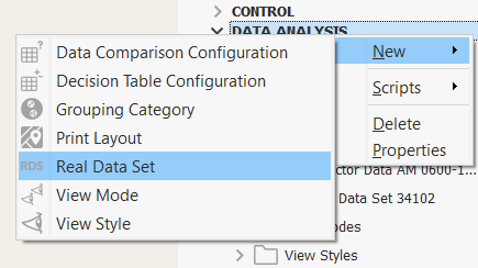
In the Project folder, right-click Data Analysis > New > Real Data Set.
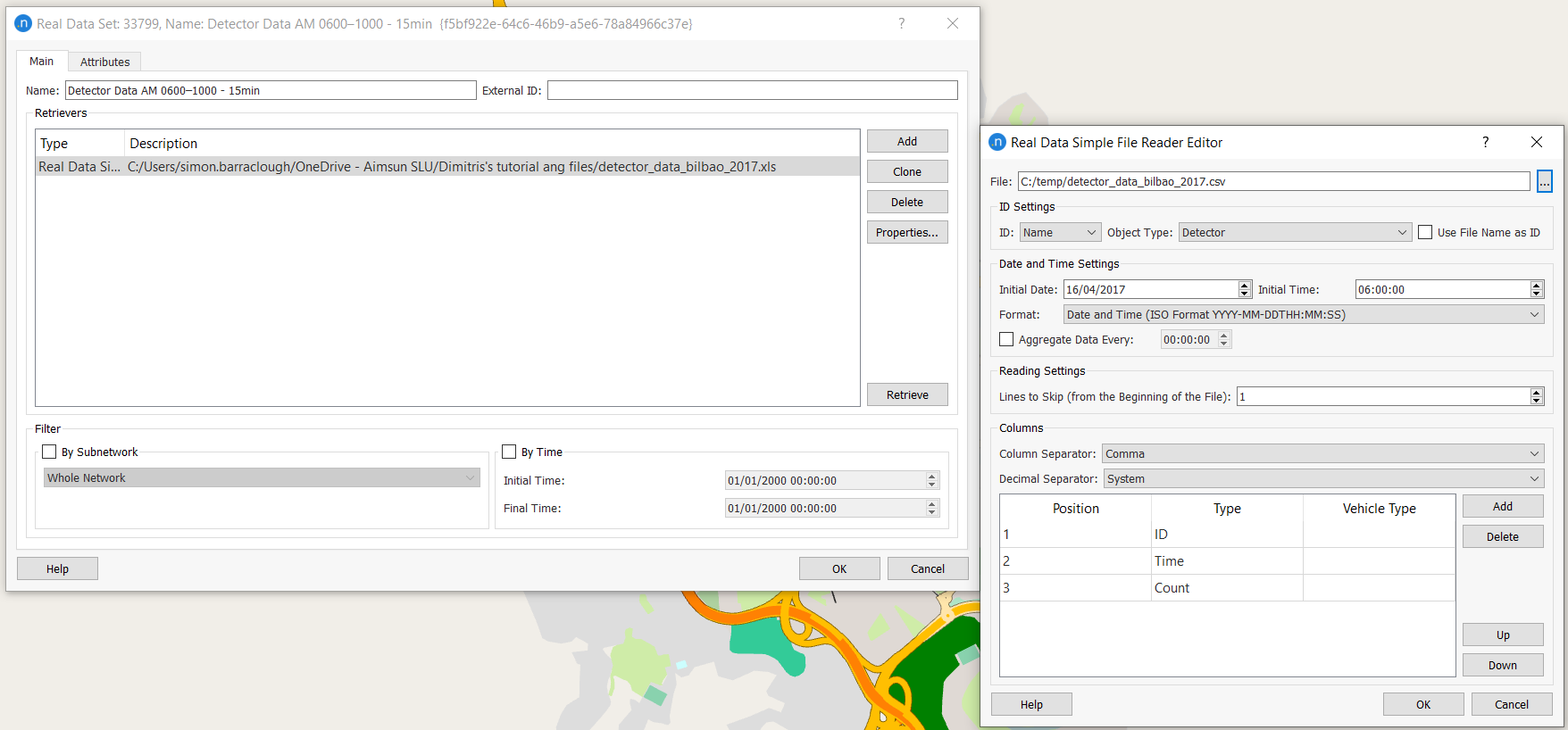
Rename the real data set Detector Data AM 0600–1000 – 15min.
Open the external file containing the detector measurements (detector_data_bilbao_2017.csv) and check the format and order of the columns in the file.

The columns are: detector_id: detector name (Aimsun Next file), timestamp: ISO format, count: number of vehicles per time interval:

detector_id,timestamp,count

d1,2017-04-16T06:15:00,585

d2,2017-04-16T06:15:00,689

d3,2017-04-16T06:15:00,480
Open the real data set Detector Data AM 0600–1000 – 15min and click Add.
From the Select a Retriever dialog, select Real Data Simple File Reader and click OK.
Double-click on Real Data Simple File Reader and complete its dialog with the inputs shown below.
Click OK.
In the Project folder, right-click Detector Data AM 0600–1000 – 15min > Retrieve. If there are no problems with the file, the RDS icon will turn blue. Any errors will be displayed in the Log window. The Check Real Data Set dialog is also displayed.

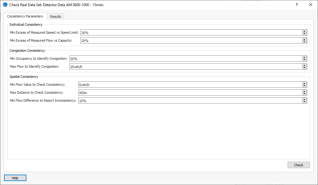
Here you can run various optional checks on the data's consistency: individual, congestion, and spatial. See Real Data Set Editing for more information.
Close the dialog by clicking the top-right × icon.

1.2 Running a static assignment scenario and experiment¶

We need to generate simulated data, with a static assignment scenario, to compare with our real data set.

Select Project > New > Scenarios > Static Assignment Scenario.
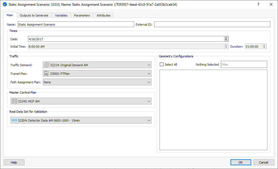
Open the new scenario to display the Static Assignment dialog.
Make sure that the date in the scenario matches the date defined in the real data set. In our illustration this is 4/16/2017 but you might be using a different date format.
For Traffic Demand, select Original Demand AM, and for Transit Plan, select Transit Plan.
For Master Control Plan, select MCP AM.
For Real Data Set for Validation, select Detector Data AM 0600–1000 – 15min.
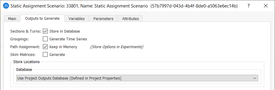
Click the Outputs to Generate tab and tick the two boxes Sections & Turns and Path Assignment.
Click OK.
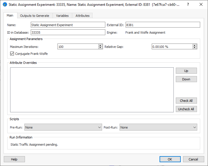
To create a static assignment experiment, in the Project folder, right-click on the new static assignment scenario and select New Experiment. Select the Assignment Method of Frank and Wolfe and click OK.
Open the static assignment experiment and enter Maximum Iterations of 100 and Relative Gap of 0.001%.

We now need to create two path assignment objects in which to store path assignment results.
In the Project folder, right-click Demand Data > New > Path Assignment to create the first object. Repeat this for the second object. You now have two new path assignment objects in which to store both path assignments (all paths and a subset of the three most-used paths per OD pair). Rename these objects Path Assignment static all and Path Assignment static 3 most used.
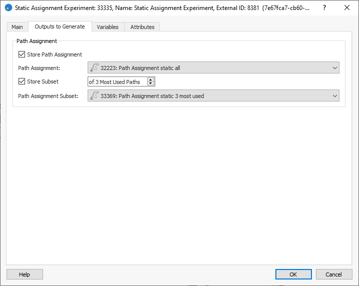
Open the static assignment experiment and click the Outputs to Generate tab. Tick the box Store Path Assignment and for Path Assignment, select Path Assignment static all. Then tick the box Store Subset and for Path Assignment Subset, select Path Assignment static 3 most used.
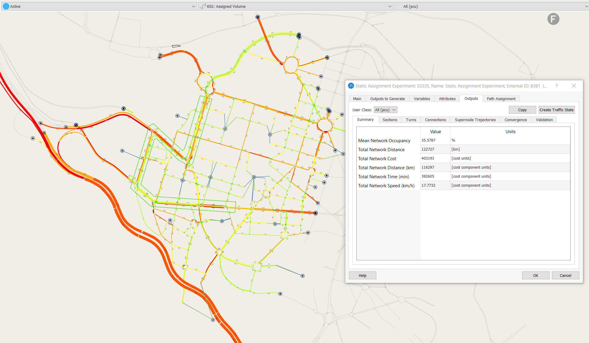
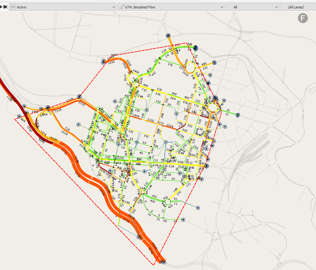
Right-click on the static assignment experiment and select Run Static Traffic Assignment. When the experiment completes its simulation, the results of the static assignment are visualized in the 2D-view window as shown below. Notice that the view mode named Assigned Volume is automatically selected. Also, a new dialog containing the static assignment results is displayed.

1.3 Comparing assigned volumes to real observed data¶

Here we will use the dialog containing the static assignment experiment results to compare our simulated data to the real data set (observed data).

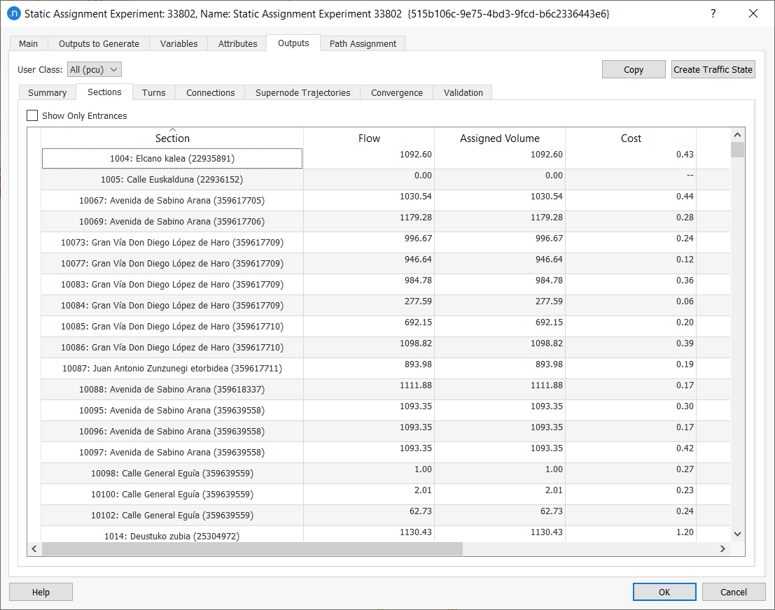
Click the Sections tab and carefully check the Flow, Assigned Volume, Cost, Distance, Speed, Time, and V/C Ratio values calculated in the final iteration. You might find it useful to sort the columns by higher or lower values. To see all values clearly, you might need to resize the dialog by clicking and dragging its edges.

Make similar checks for the following tabs: Turns, Connections, and Supernode Trajectories.
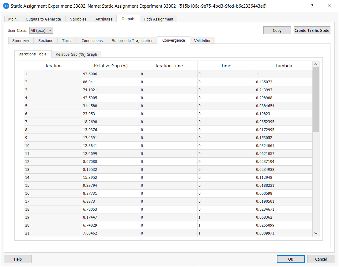
Click the Convergence tab and verify that the Relative Gap % (available in both table and graph mode) is sufficient, according to the requirements of the project.
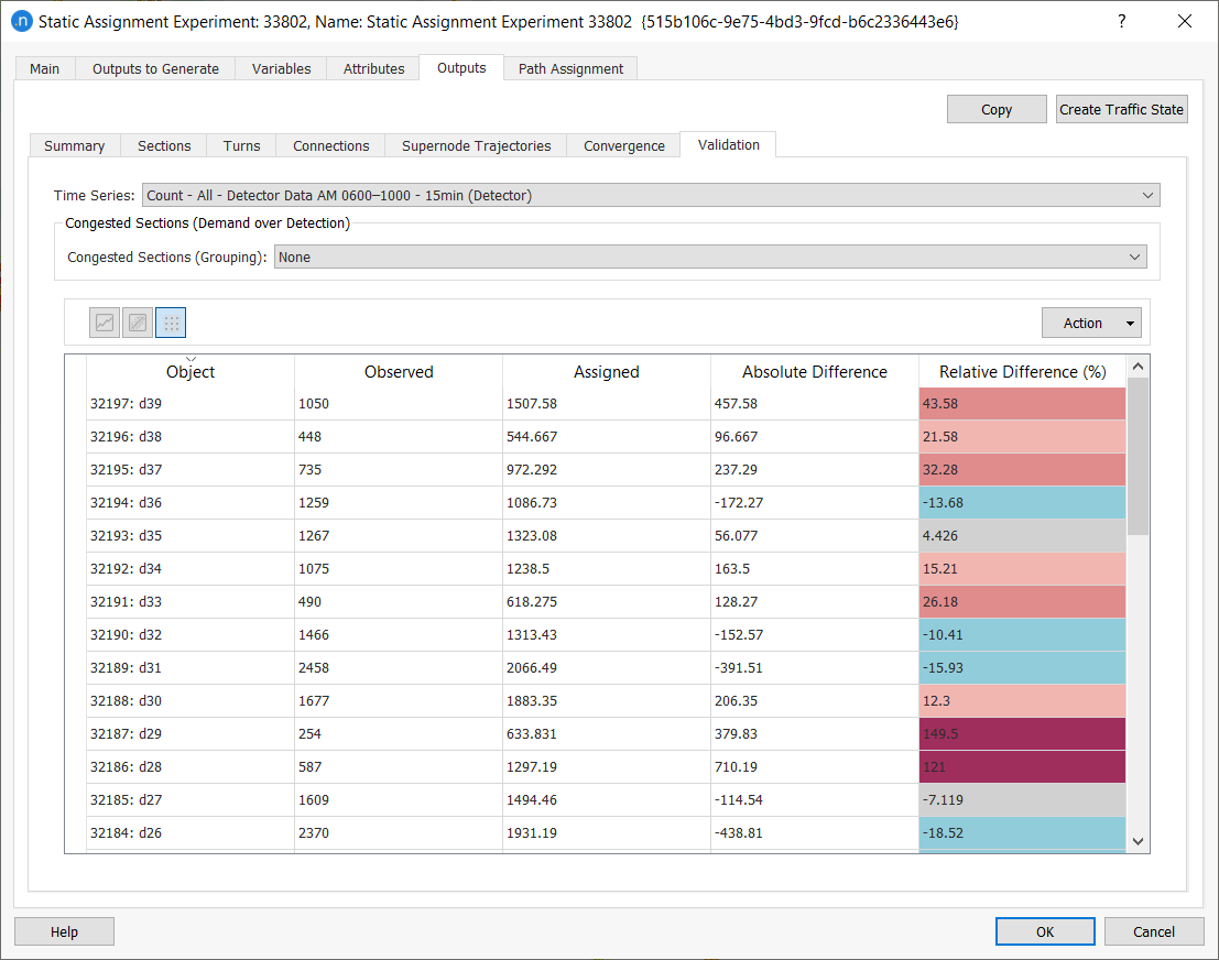
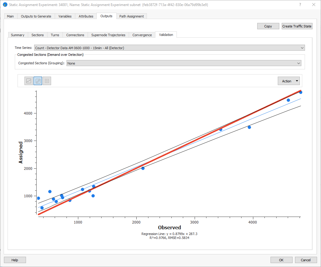
Click the Validation tab and compare the results with the real data set Detector Data AM 0600–1000 – 15min.
Click to view the distribution of assigned versus observed flows between 08:00 and 09:00.

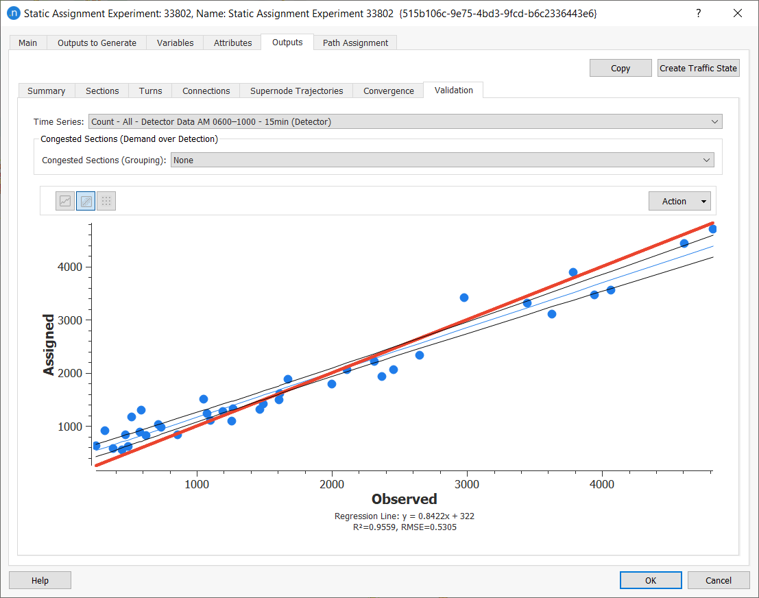
In terms of results, initially we obtain an R² value of 0.96, which shows that there is a high degree of correlation between the observed and assigned values. This is a good result. However, the slope of the line is below 1.00, with a value of 0.85 (rounded up). We can see from the red line, which indicates y = x, that the observed counts (rds) in detector locations are:

For low volumes (< 2000 veh): lower than the assigned volumes
For high volumes (> 2000 veh): higher than the assigned volumes.

This happens because the current observed counts (rds) were obtained in 2017 while the traffic demand OD matrices data were based on a 2010 survey. Also, the model was validated with more recent data from 2013. Since then, there have been a few changes in the traffic routes between 08:00 and 09:00: traffic usage on highways has decreased, while the traffic on arterial roads has increased.

This macroscopic model is considered sufficiently calibrated in terms of global and local parameters used in the VDF, TPF, and JDF functions.

Next we need to define a subnetwork as our ongoing study area.

Exercise 2. Defining a Subnetwork Study Area and Running a Static Traversal¶

To focus our study on the area around the scheme, we will create a subnetwork and run a static traversal. This will create the OD matrices for the subnetwork. In a real-world project, we would consider the following types of information provided by external sources and then:

Review the project documentation to check that the proposed study area is properly defined.
Verify the congested sections of the study area. Because congestion at model boundaries should be avoided, we might need to extend the study area around some entrances and/or exits of the model.
Check the current map of detectors in the study area. We need to include the maximum number of detectors in the study area and might need to extend the area of the subnetwork in some cases.

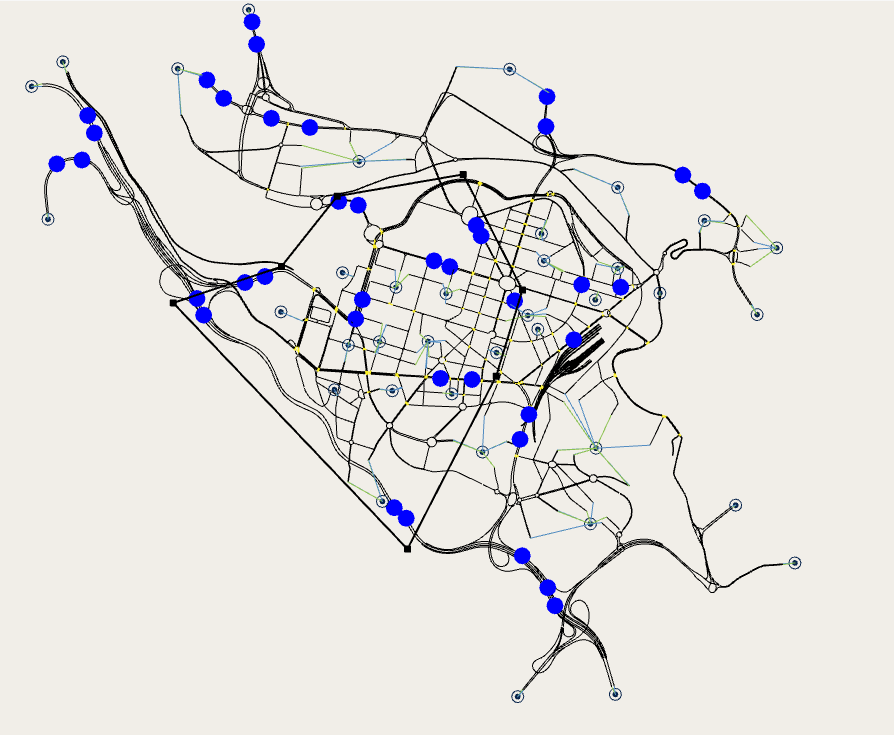
In our example, let's assume that after a discussion with the client and third parties we finalized the study area shown below. The area is marked out by a black polygon with square vertices.

2.1 Defining a subnetwork¶

Click the polygon tool on the toolbar.

Draw the polygon by clicking its vertices at the required points. To finish and close the polygon, double-click to add the final point.
Click on the polygon in the 2D view to highlight it and then right-click Convert to > Subnetwork. A subnetwork object is added to the Project folder in the Subnetworks folder.
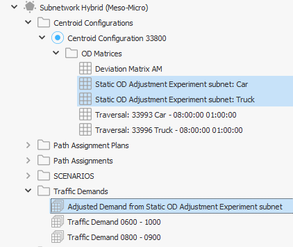
Open this new subnetwork object and rename it Subnetwork Hybrid (Meso-Micro). You can also rename objects by clicking on their names in the relevant folder and pressing F2.

2.2 Running a static traversal¶

In this exercise we will generate a static traversal to create the OD matrices for the subnetwork. The new OD matrices will be based on the static assignment results generated in Exercise 1.

We will then run a static assignment scenario of the subnetwork and review the traversal matrix outputs.

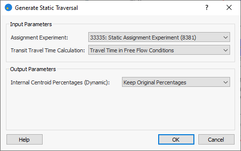
In the Project folder, right-click Subnetwork Hybrid (Meso-Micro) > Generate Static Traversal.
In the traversal dialog, select the input parameters shown below and click OK.

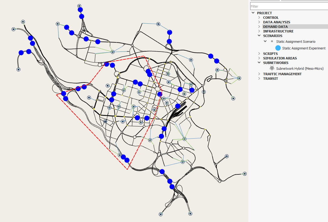
OD matrices (for car and truck), traffic demands, and transit lines with the transit plan will be automatically generated for the subnetwork and added to the Subnetworks folder, as shown below.
To highlight the subnetwork in the 2D view, right-click anywhere in the 2D view and select Filters > Subnetwork Hybrid (Meso-Micro).

To verify the static traversal demand, we will test them in a new static scenario.
In the Project folder, right-click Subnetwork Hybrid (Meso-Micro) > New > Scenarios > Static Assignment Scenario.
Rename the scenario Static Assignment Scenario subnet.
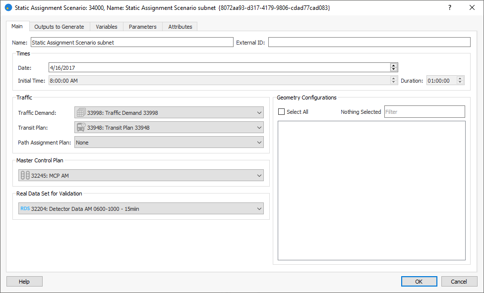
Open Static Assignment Scenario subnet, complete the parameters on the Main tab as shown below, and click OK.
Right-click on the scenario and select New Experiment, select the Assignment Method Frank and Wolfe, and click OK.
Open the experiment, rename it Static Assignment Experiment subnet and set the number of iterations and stopping criteria as in Exercise 1 (Max. Iterations 100, Relative Gap 0.001%).
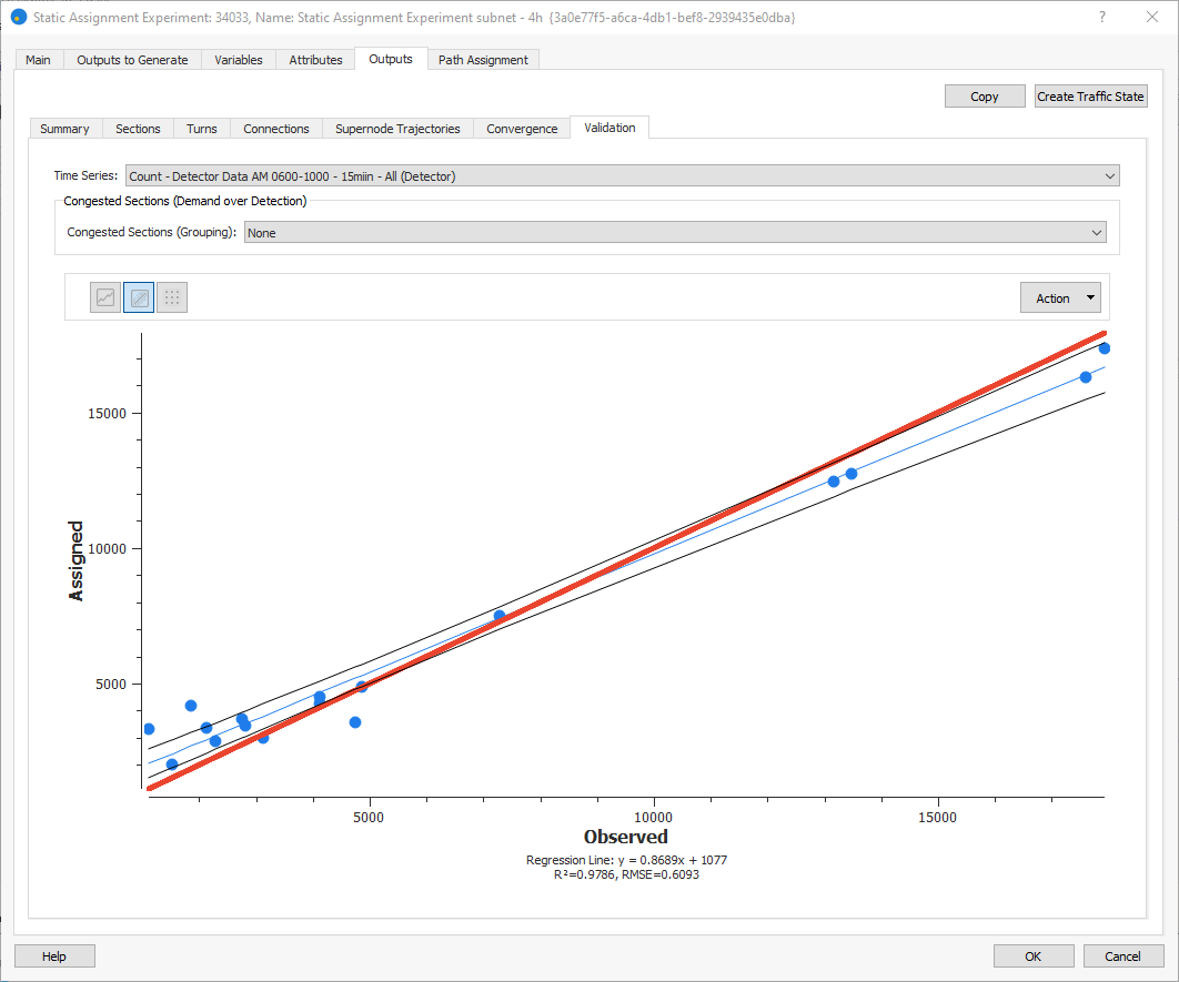
Right-click on the experiment and select Run Static Traffic Assignment. When it is finished and the results dialog is displayed, click the Validation tab to check the comparison between the real-data counts and the results of the assignment. The static assignment result looks consistent with the results from the larger model.

Exercise 3. Checking Detection Coverage¶

It is important to know whether the available detection data sufficiently covers the traffic network conditions in the subnetwork. To find out, use the Detector Location feature to check the current coverage of detectors. This knowledge can help you decide whether to move, or add new, detectors to the network to cover all relevant conditions. In a real-life project, economic and other practical factors might influence decisions about the number and location of detectors.

For step 5, you need to know the names of detectors in the subnetwork. You can see them by switching to the view mode Detectors in the 2D view.

In the Project folder, right-click Infrastructure > New > Detector Location. A detector location object is added to the Infrastructure folder.
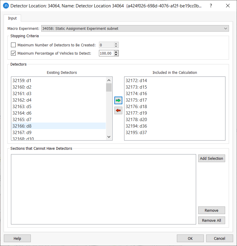
Open the detector location and, in the Macro Experiment field, select Static Assignment Experiment subnet.
Tick Maximum Percentage of Vehicles to Detect and set the value as 100.00. For a real-life project, this value might be smaller due to economic reasons or other project restrictions and guidelines.
In the Detectors group box, select the detectors in the subnetwork from the Existing Detectors column and click the green arrow to move them into the Included in the Calculation column.
Click OK.
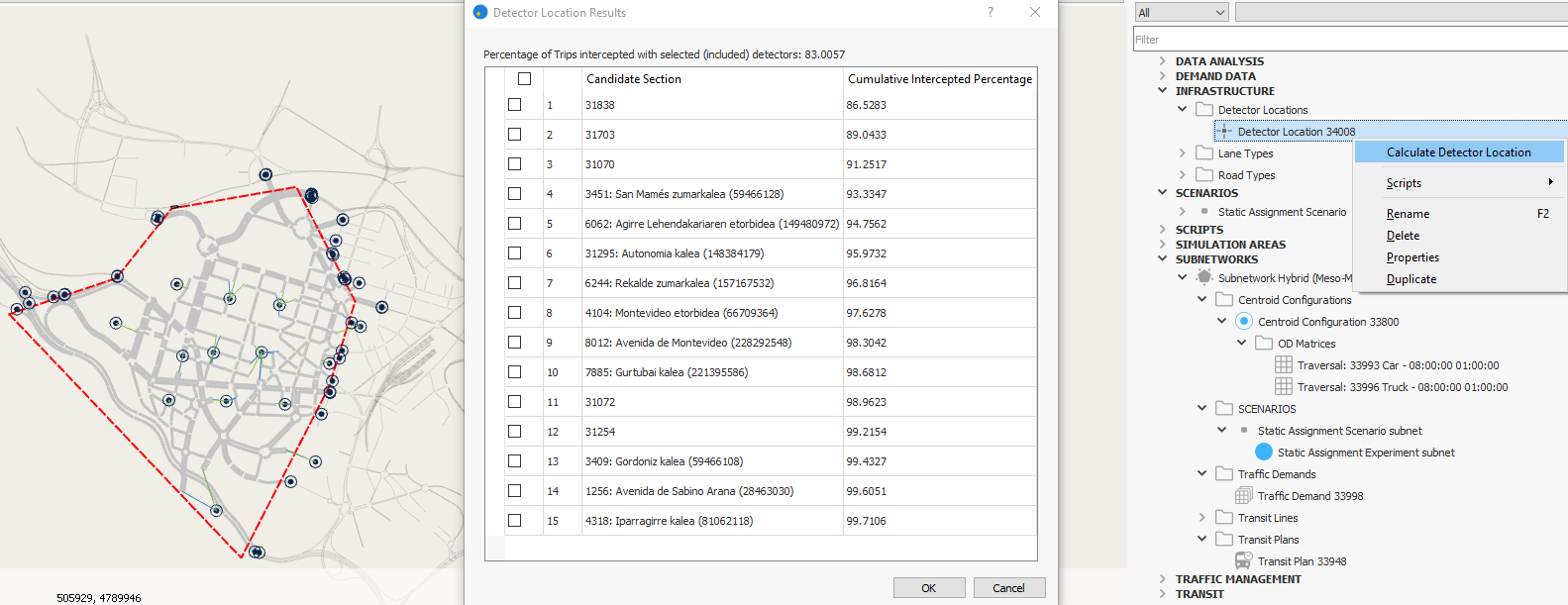
In the Project folder, right-click Detector Location > Calculate Detector Location to show the results.

According to the results below, the percentage of detection coverage is around 87% and upwards, which is considered sufficient in this particular case.

Exercise 4. Extending the OD Matrices Based on Traffic Measurements¶

Because the observed counts in the real data set include four hours' worth of data from 06:00 to 10:00, with a time interval of 15 minutes, we need to extend the one-hour available traffic demand to cover a four-hour period. To do so, we need to calculate the weight coefficient to extrapolate from the original traffic demand, which equals 27,611 vehicles.

In 4.2 we will apply the extended matrices to a scenario.

4.1 Extending the OD matrices¶

Divide the total trips of the observed counts from 06:00 to 10:00 am (246,372 veh) by the total trips of the observed counts from 08:00 to 09:00 am (67,590 veh):

246,372 ÷ 67,590 = 3.65 (rounded up).

So the resulting weight needed to multiply the seed OD matrices of the original traffic demand is 3.65 (a factor of 365).
Make a copy of the subnetwork traffic demand by right-clicking on it and selecting Duplicate.
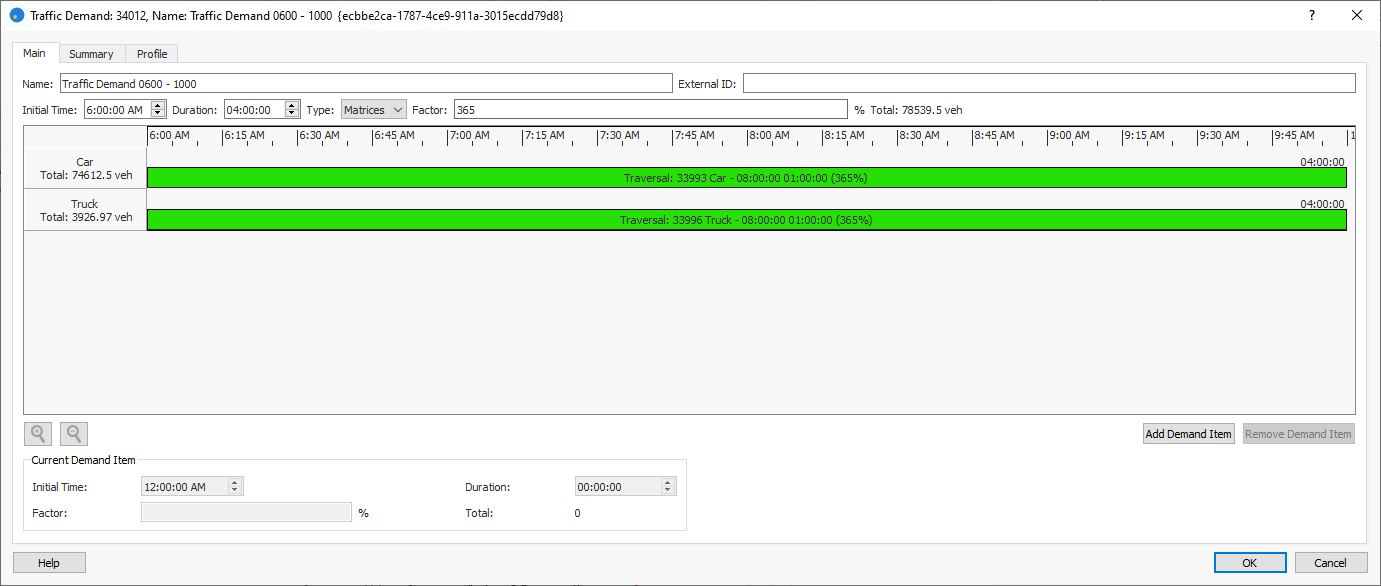
Open the new traffic demand object and rename it Traffic Demand 0600–1000.
Change Initial Time to 06:00:00 and Duration to 04:00:00.
Press the Tab key to move to the adjacent Factor field and enter 365. Press Tab again to apply the factor.
Click and drag each of the green demand bars for Car and Truck to the full extent of the duration.
Click OK.

4.2 Using the extended OD matrices with a static assignment scenario¶

Right-click on the existing scenario Static Assignment Scenario subnet > Duplicate. This places copies of the scenario and its experiment in the Subnetworks folder.
Rename the duplicated scenario and experiment Static Assignment Scenario subnet – 4h and Static Assignment Experiment subnet – 4h respectively.
Open Static Assignment Scenario subnet – 4h and, for Traffic Demand, select Traffic Demand 0600–1000 and click OK.
Right-click Static Assignment Experiment subnet – 4h > Run Static Traffic Assignment. Check the results as we did in Exercise 2.2.

Exercise 5. Adjusting the subnetwork OD matrices¶

Because the OD matrices we have used so far are based on data from 2013, we need to adjust them so that they align more closely with the real data set from 2017. To do this, we will run a static OD adjustment scenario on the OD matrices and then run a new experiment.

5.1 Running a Static OD Adjustment Scenario¶

Right-click on the subnetwork Subnetwork Hybrid (Meso-Micro) > New > Scenarios > Static OD Adjustment Scenario.
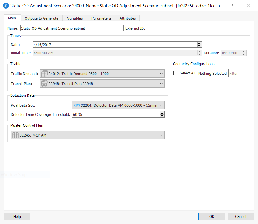
Open the new scenario and rename it Static OD Adjustment Scenario subnet.
Set the Date, Initial Time, Duration, Traffic Demand, Transit Plan, Real Data Set, and Master Control Plan as shown below.
Right-click on the subnetwork and select New > Path Assignment.
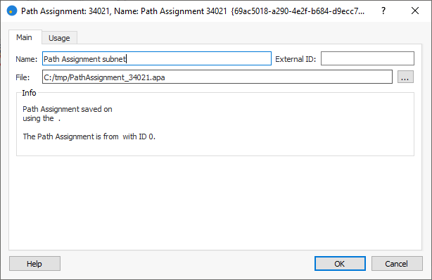
Open the new path assignment object and rename it Path Assignment subnet.
In the File field, browse to and add the path assignment file PathAssignment_34021.apa (quick reminder: files can be found in Aimsun_Next_Installation_Folder]/docs/tutorials/7_Integration]).
Below Subnetwork Hybrid (Meso-Micro) right-click Centroid Configuration > New > OD Matrix.
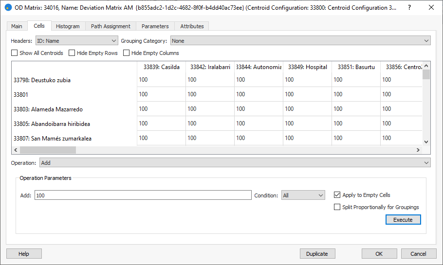
Open the OD matrix and rename it Deviation.
In the Contents field, select Maximum Deviation.
Click the Cells tab and for Operation, select Add.
In the Add field, enter 100, for Condition, select All, and tick the Apply to Empty Cells box.
Click Execute.
Click OK.

5.2 Running a new static OD adjustment experiment¶

Right-click on the static OD adjustment scenario and select New Experiment. Accept the Assignment Method of Frank and Wolfe and click OK.
Open the experiment, rename it Static OD Adjustment Experiment subnet, and click the Adjustment Constraints tab.
In the Demand Elasticity group box, set the Matrix Elasticity factor to 0.55.

This parameter controls by how much the values in the adjusted matrix might vary as the adjustment scenario proceeds.
In the Demand Bounds group box, select the Deviation matrix for both Car and Truck.
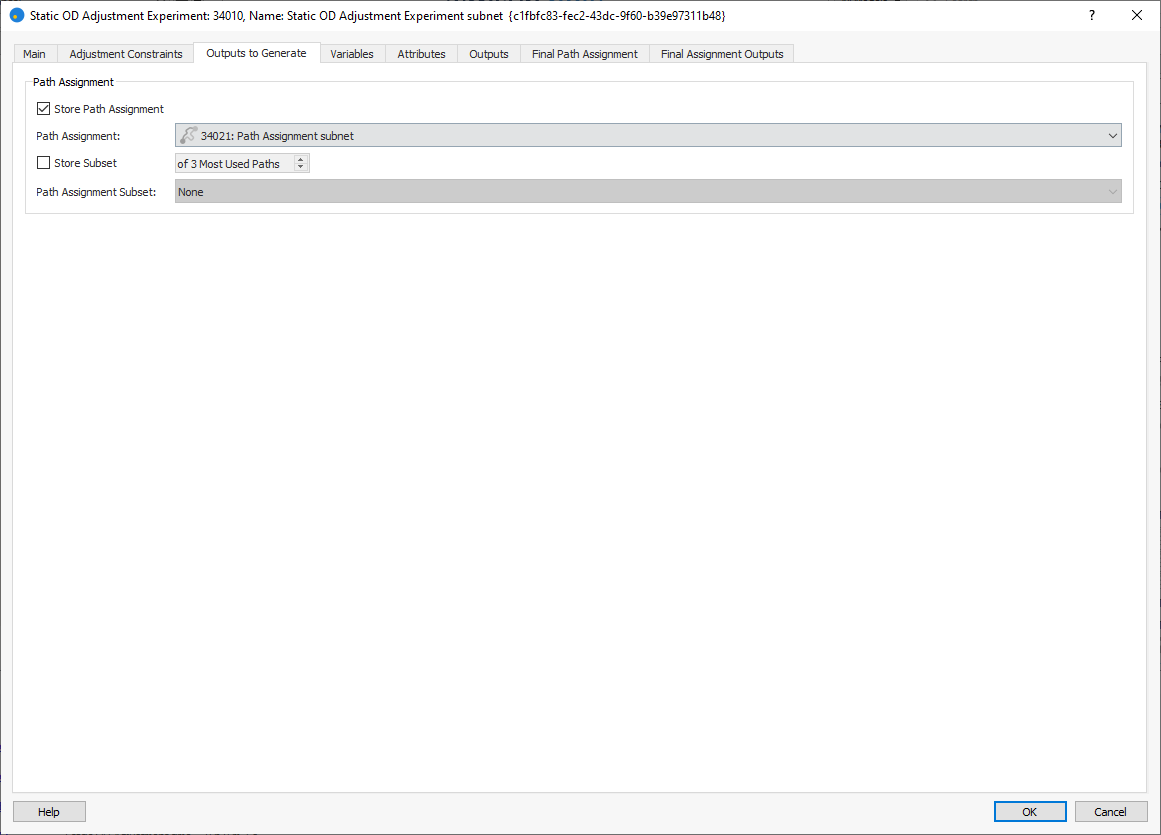
Click the Outputs to Generate tab, tick the box Store Path Assignment, and select the path assignment file that we created in Exercise 5.1.
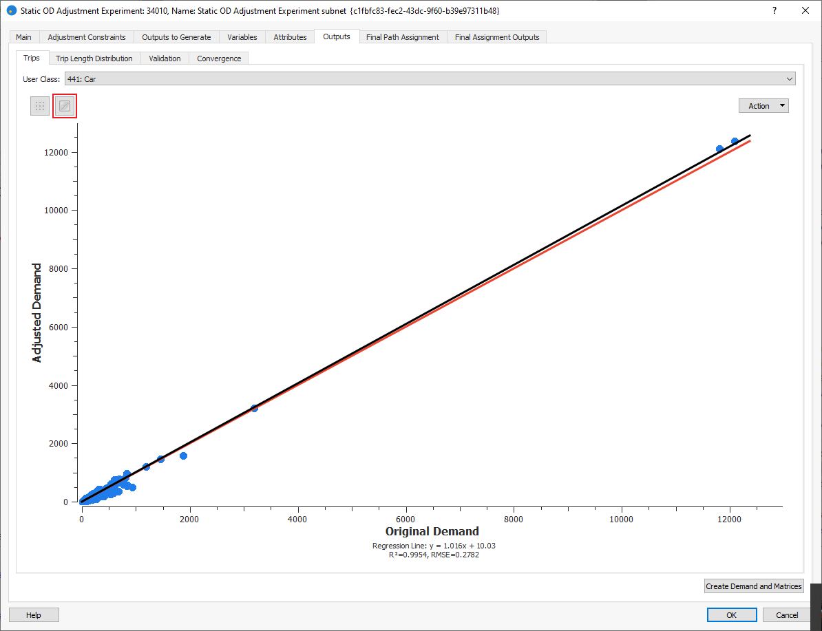
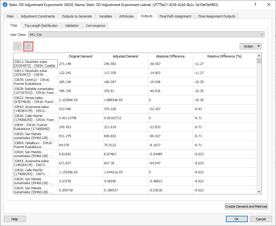
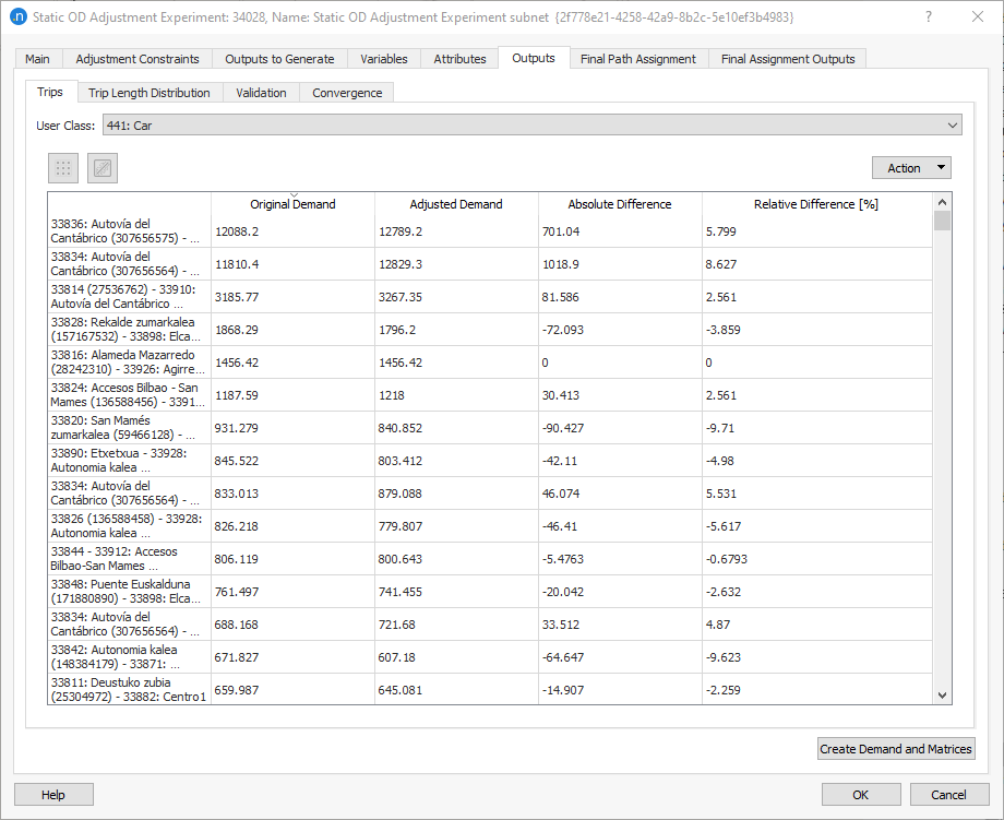
Right-click Static OD Adjustment Experiment subnet > Run Static OD Adjustment. On the results dialog, click the Outputs tab and then on the Trips subtab compare the number of trips for each OD pair before and after the assignment. You might need to click the graph icon first.
Click the table icon and sort by Relative Difference [%] to verify that the maximum and minimum values are under +-100%.
Sort by Original Demand and verify that the OD pairs have been modified as desired. If a specific OD pair has changed more than the desired value, you can find the OD pair in the Deviation matrix and reduce the value from 100% to, for example, 50%.
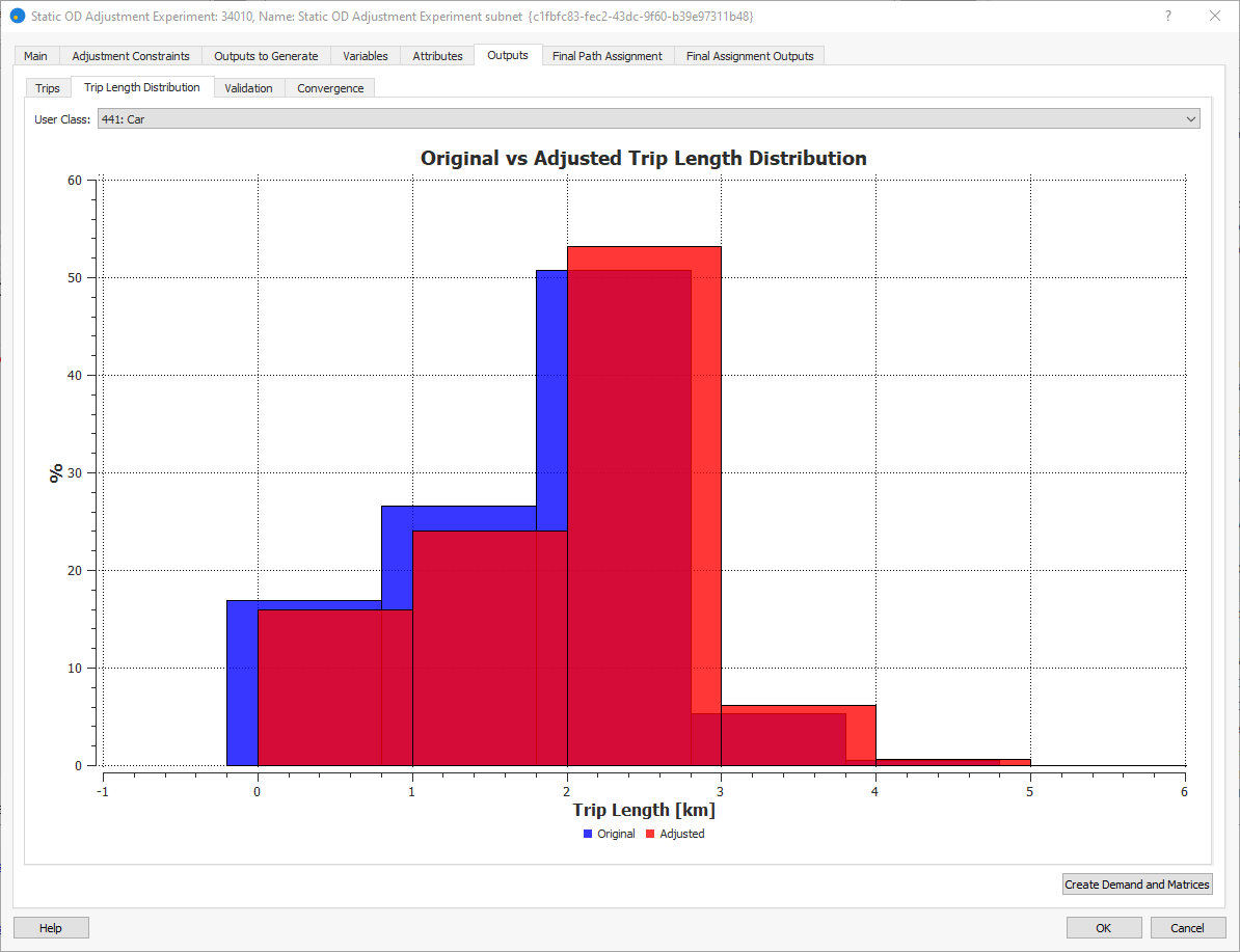
Click the Trip Length Distribution tab. The result looks good, so there is no need to modify Matrix Elasticity or Trip Length Distribution.
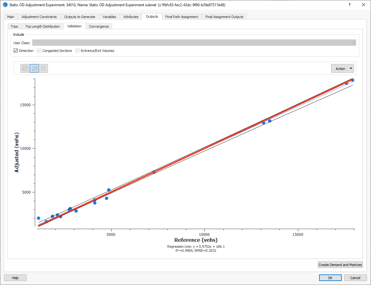
Compare the assignment outputs with the observed counts from 06:00 to 10:00. Click the Validation tab and, as with the assignment process, check the regression line graph. The number of OD trips has reached the observed counts.

Now we can create the adjusted traffic demand objects.
Click Create Demand and Matrices and check that three new objects have been created. These should be two new four-hour OD matrices (car, truck) and one traffic demand with the new OD matrices assigned to it.

Exercise 6. Creating a Profiled Demand with a Static OD Departure Adjustment¶

To obtain the required profiled demand, the static flat demand from 06:00 to 10:00 needs to be distributed through smaller intervals across the time period. A Static OD departure adjustment can be used to profile the original static matrix automatically. We want to reproduce the observed traffic counts specified in the real data set per interval, staying as close as possible to the original number of OD-pair trips for the whole period.

It is important to start the process with a calibrated demand that fits the detection data of the full modeled period. The static OD departure adjustment does not calculate any new assignment; it takes previously calculated fixed paths from a path assignment produced earlier, plus link (section + turn) travel times and uses them to calculate the assigned number of vehicles for each time period.

Right-click Subnetwork Hybrid (Meso-Micro) > New > Path Assignment Plan.
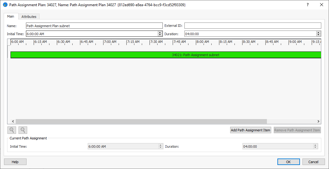
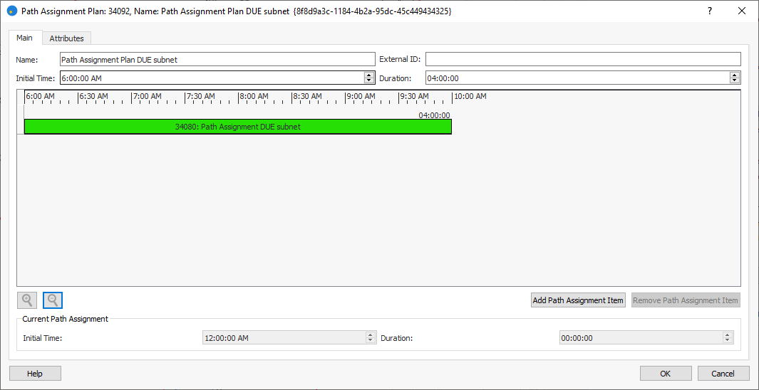
Open the new plan, rename it Path Assignment Plan subnet, and set the Initial Time to 06:00:00 and Duration to 04:00:00.
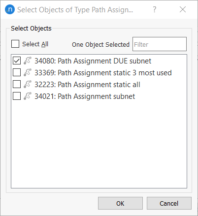
Click Add Path Assignment Item and, on the Select Objects of Type dialog, tick Path Assignment subnet.
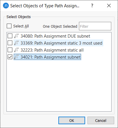
Click OK to add the path assignment to the Path Assignment Plan dialog.
To add the required scenario, right-click Subnetwork Hybrid (Meso-Micro) > New > Scenarios > Static OD Departure Adjustment Scenario.
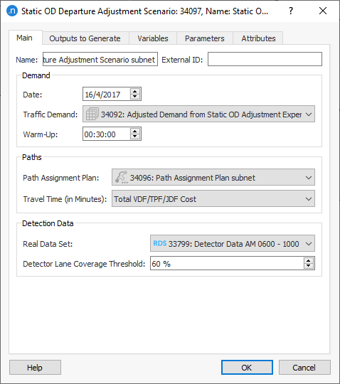
Open the scenario, rename it Static OD Departure Adjustment Scenario subnet, and set the attributes as shown below.
Right-click on the scenario and select New Experiment.
Open the experiment, rename it Static OD Departure Adjustment Experiment subnet and, in the Demand Bounds group box, make sure that the Max Deviation Matrix column contains both Car and Truck matrices.
For Max Deviation Value, select Percentage.
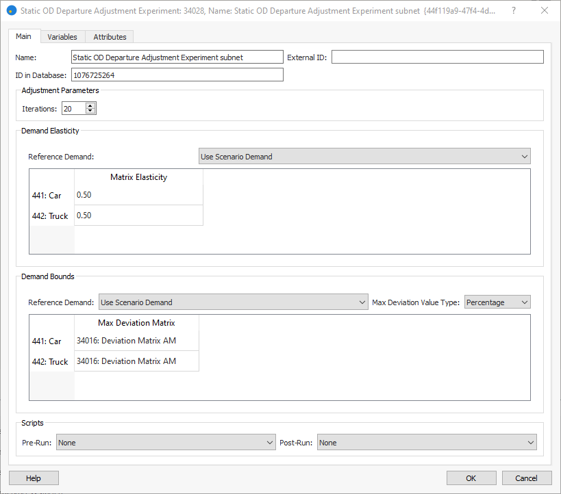
Click OK.
Right-click Static OD Departure Adjustment Experiment subnet > Run Static OD Departure Adjustment.
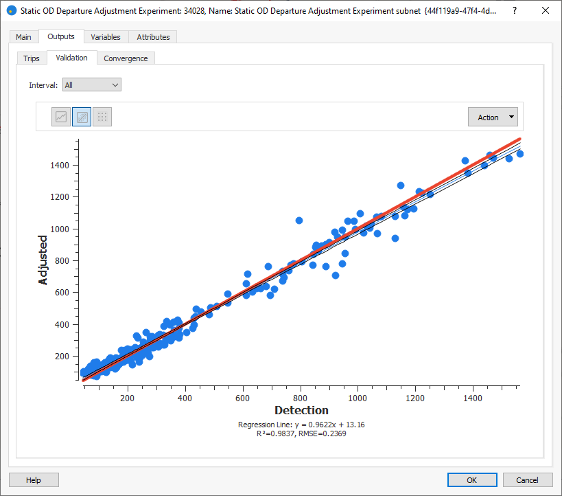
Once it is finished and the results dialog is displayed, view the Trips and Validation tabs. Check the regression line graph results per interval to verify the result for all intervals.
Click the Trips tab again and click Create Demand and Matrices. Many new profiled matrices are created and added to the Project folder in the Subnetworks folder.

Exercise 7. Running a Mesoscopic Dynamic User Equilibrium (DUE) Experiment, Loading Static Paths¶

In this exercise we will run a DUE mesoscopic simulation to obtain a new set of paths. We will be using the subnetwork we created in Exercise 2 and the profiled traffic demand from 06:00–10:00.

Double-click on the profiled traffic demand from the previous exercise and, for both items Car and Truck, select the intervals 05:30–05:45 and 05:45–06:00 as illustrated below (hold the Shift key to select multiple items).
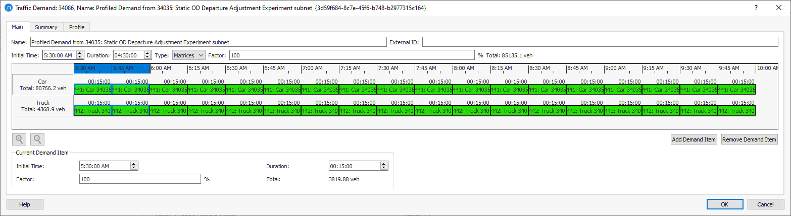
Click Remove Demand Item to delete your selection and click OK. The profiled traffic demand now starts at 06:00 with a 4-hour duration.
Right-click Subnetwork Hybrid (Meso-Micro) > New > Scenarios > Dynamic Scenario.
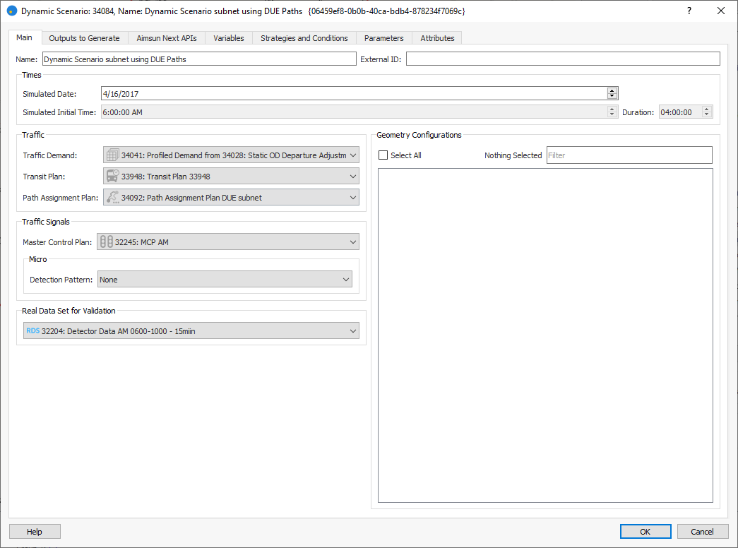
Open the scenario, rename it Dynamic Scenario subnet, and complete its parameters as shown below.

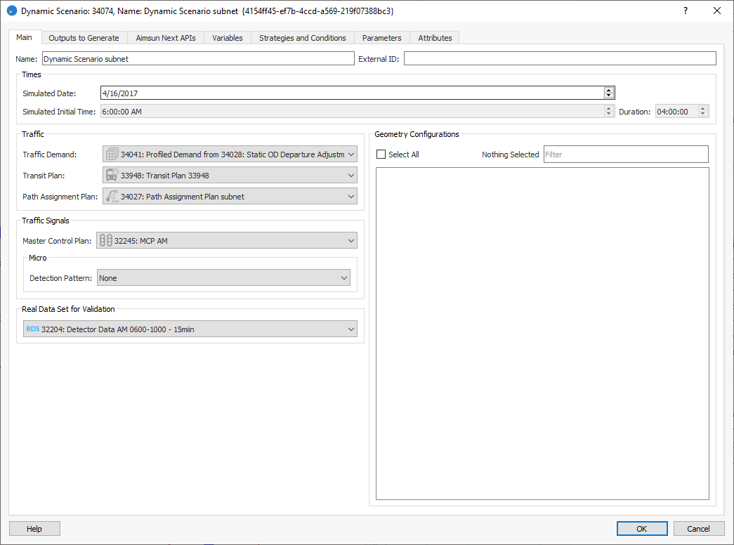
Note that it will use the adjusted traffic demand from the static OD departure adjustment experiment and the path assignment plan from the Static OD Adjustment Experiment subnet, which was run using the 06:00–10:00 flat demand.
Right-click on the scenario and select New Experiment.
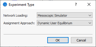
In the Experiment Type dialog, for Network Loading, select Mesoscopic Simulator, and for Assignment Approach, select Dynamic User Equilibrium Assignment.
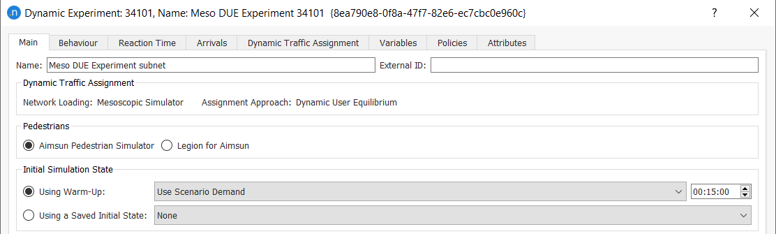
Open the experiment and rename it Meso DUE Experiment subnet.
On the Main tab, set the Using Warm-Up period to 00:15:00 minutes, so that the simulation starts with traffic already circulating throughout the network.
Click the Dynamic Traffic Assignment tab. In the Dynamic User Equilibrium group box, for Do Not Consider Paths with a Percentage Below, enter 3.00. This means that only paths with more than a 3% share over the total share-per-OD will be taken into account during the iterations of the DUE process.
Click OK.
Right-click on the subnetwork and select New > Path Assignment.
Rename the new path assignment object Path Assignment DUE subnet. This is where path assignment statistics will be stored.
Right-click Meso DUE Experiment subnet > New > Result.
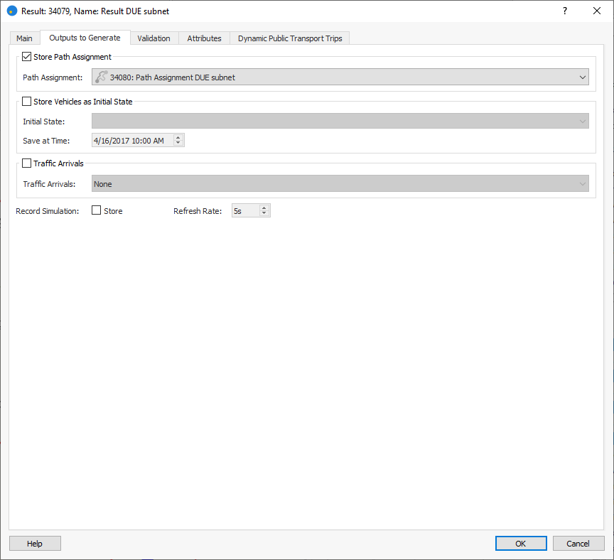
Open the result and rename it Result DUE subnet.
Click the Outputs to Generate tab and tick the box Store Path Assignment and, in the Path Assignment field, select Path Assignment DUE subnet.
Right-click Result DUE subnet > Run Batch Simulation. The Simulation Control Bar is displayed at the top of the main window while it is running.
Optional: Click the information icon [‘i’] to show the Result dialog (in progress) and click the Relative Gap tab to see the evolution of the relative gap for each time slice (determined by the route-choice cycle time).
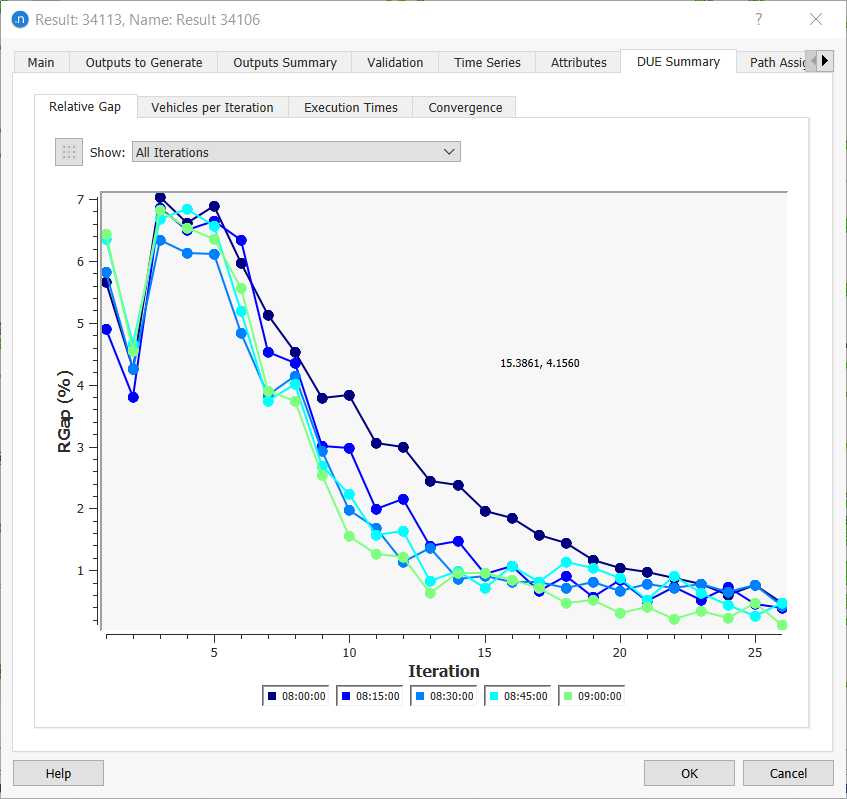
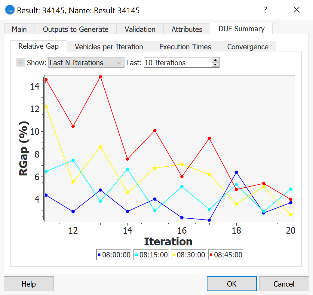
When the simulation has finished, click the DUE Summary tab on the Result dialog to check, by color, the RGap (%) per interval as calculated after each iteration. Each interval reaches the stopping criteria that was set (RGap = 0.5%).
Click the Vehicles per Iteration tab to check the number of vehicles that are: Waiting to Enter, Inside, or Outside (have already left) the network per iteration. This indicates whether there are any potential gridlocks in the simulation that might cause unexpected virtual queues.
Click the Validation tab to check the quality of the simulation in terms of counts. Check the regression line graph results to validate the result for each interval.

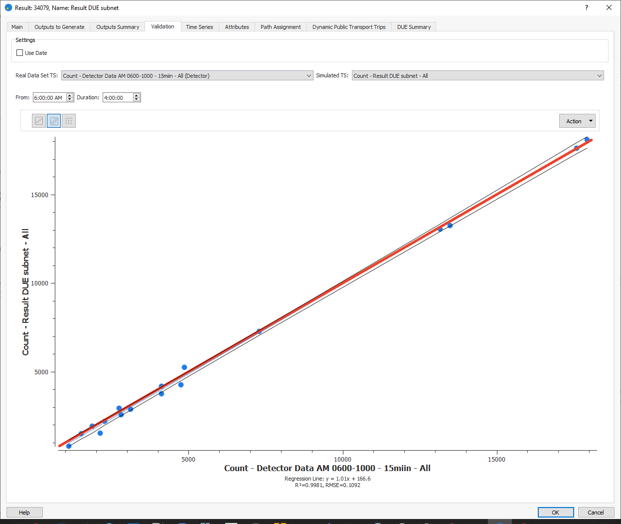
Because there is no information about the congested sections in the network, in a real-world project we might need to ask for this information to be provided so that the model emulates real traffic conditions. This applies not only to counts but also to speed and/or delay times.

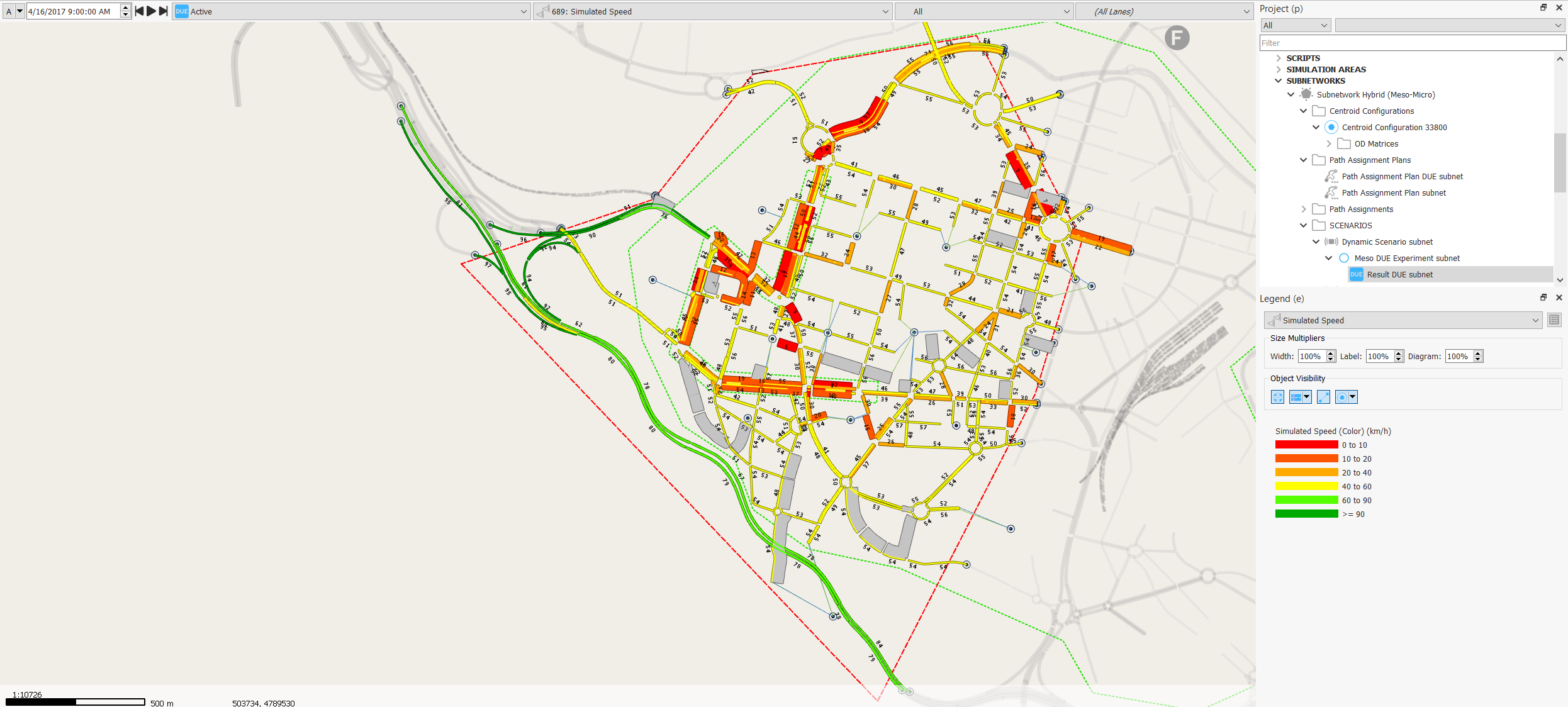
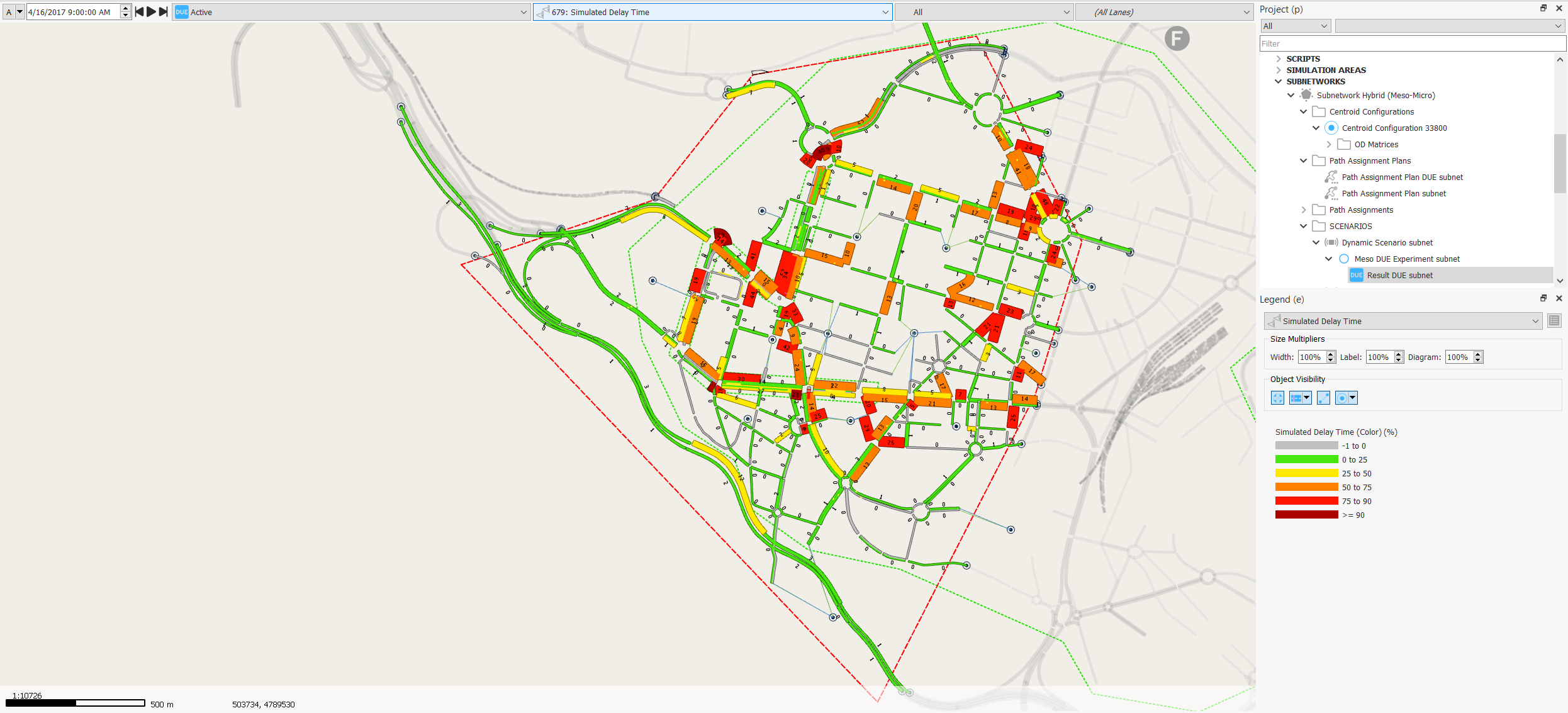
To check global traffic conditions in the model, select the view modes Simulated Speed and Simulated Delay Time and play back the simulation for each view mode to visualize results in 15-minute increments. Note, at 07:30, the speed and delay times represented in different colors for every section based on the legend provided with the view mode.

Exercise 8. Running a Microscopic Stochastic Route Choice (SRC) Scenario, Loading DUE Dynamic Paths¶

In this exercise we will simulate a microscopic SRC experiment, using a percentage of the paths generated from the previously obtained DUE results. First, we will set up the scenario and experiment, then we will check and compare the results.

8.1 Setting up the scenario and experiment¶

Right-click Subnetwork Hybrid (Meso-Micro) > New > Path Assignment Plan.
Open the new path assignment plan and set the Initial Time as 06:00:00 with a Duration of 04:00:00 (till 10:00:00).
Click Add Path Assignment Item and, on the Select Objects of Type dialog, tick Path Assignment DUE subnet.
Click OK to add the path assignment to the Path Assignment Plan dialog.
Right-click Subnetwork Hybrid (Meso-Micro) > New > Scenarios > Dynamic Scenario. This scenario will use DUE paths.
Open the new scenario and rename it Dynamic Scenario subnet using DUE Paths.
On the Main tab, complete the parameters as shown below. This ensures that the adjusted OD matrix and the paths from the DUE experiment we ran in Exercise 7 are used.
Right-click on the scenario and select New Experiment.
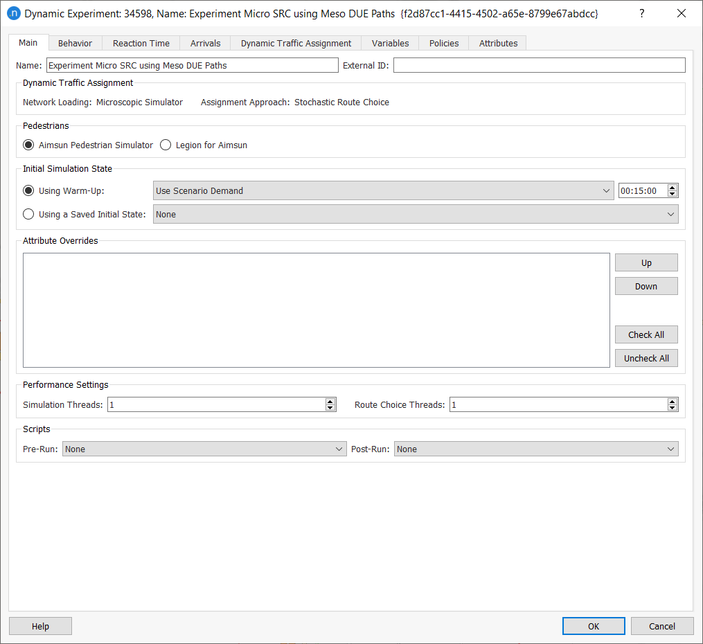
Open the experiment and rename it Experiment Micro SRC using Meso DUE Paths. On the Main tab, complete the parameters as shown below.
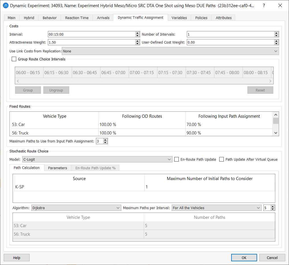
Click the Dynamic Traffic Assignment tab and complete the following parameters.

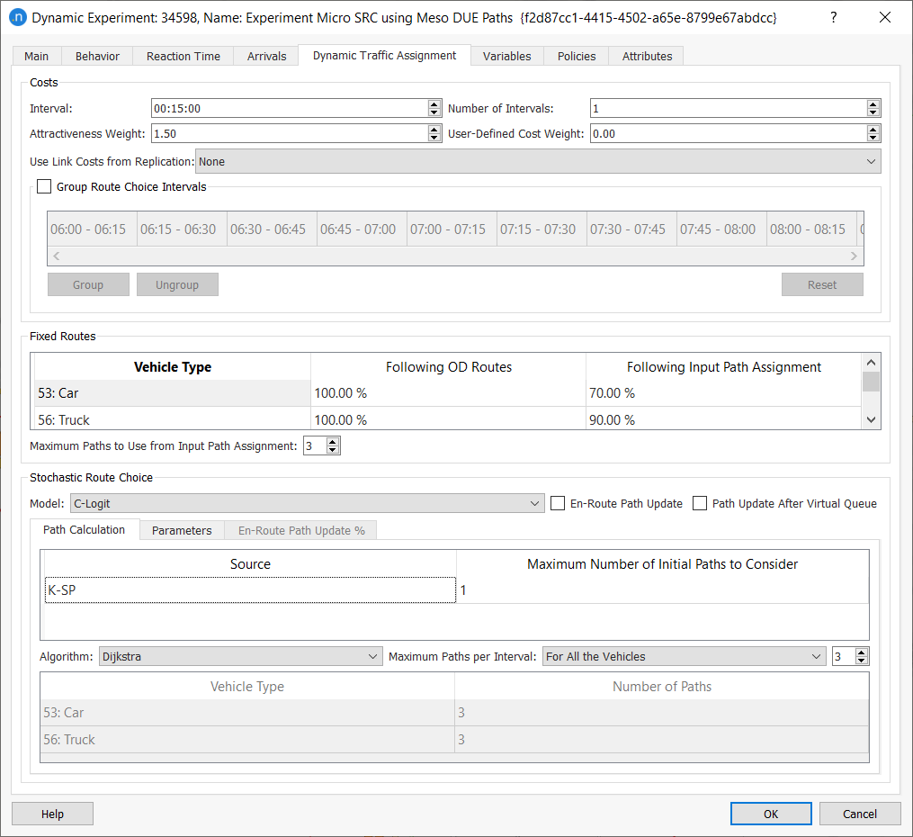
The Fixed Routes group box indicates that 70% of cars and 90% of trucks will follow the path assignment. The remaining trips will follow the OD routes that are calculated based on the dynamic cost functions which update the costs after every interval (in this case, 15 minutes).

Lower down on the dialog, the Maximum Paths to Use from Input Path Assignment value is 3 and the Maximum Paths per Interval is 5. This means that two alternative paths will be calculated as well as the three paths available per OD pair in the path assignment file (totaling 5).
Right-click on the experiment and select New > Replication.
Open the replication and rename it Replication Experiment Micro SRC using Meso DUE Paths.
Right-click Replication Experiment Micro SRC using Meso DUE Paths > Run Batch Simulation.
Check the Log window at the bottom of the 2D view to verify that the path assignment results have been retrieved from the corresponding path assignment file.

8.2 Checking and comparing the results¶

When the replication is complete and the dialog containing results is displayed, click the Validation tab and then .

As well as the R² plot and the slope, check the root mean square error (RMSE) criteria, which is 0.08595 here. The smaller the RMSE, the better the model fits.

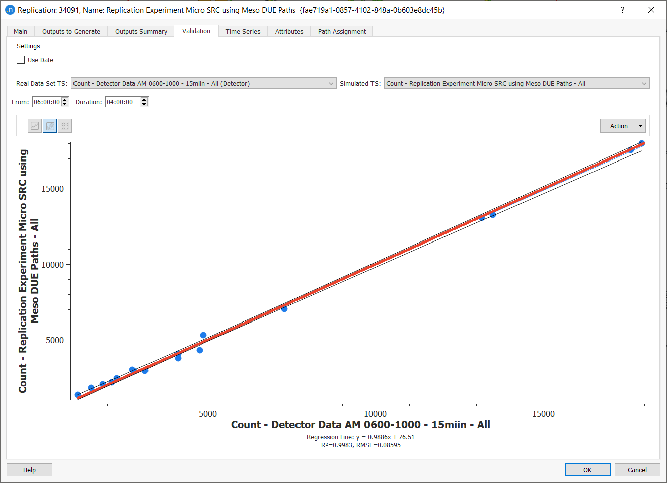
Another validation criteria that is commonly used is the GEH formula, which compares hourly traffic counts to hourly simulation outputs.
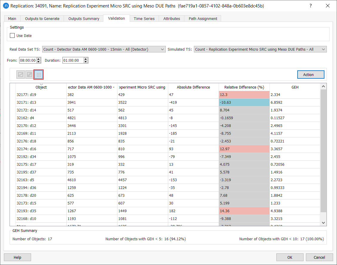
Staying on the Validation tab, change From to 08:00:00 and Duration to 01:00:00.
From the Action drop-down menu, select Calculate GEH to calculate the formula for the AM peak hour.

A view mode named GEH Statistic for 34091: Replication Micro SRC using Meso DUE Paths is created and displayed. You might need to move the replication results dialog to see the view mode better. This view visualizes, using a color range, the quality of the detectors' data. Display the Legend for further details (if it isn't visible, click in the 2D view and type e).
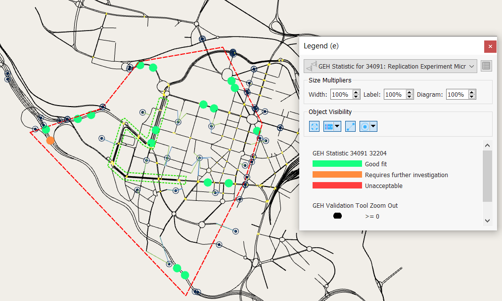
Click the table icon and check the GEH Summary at the bottom of the Validation tab. The quality of the GEH criteria of this simulation is acceptable (GEH < 5: 16 (94.12%)). In most projects, the minimum GEH criteria is defined as GEH < 5: 85.00%. If you want to make further checks, you can verify that all hourly intervals meet the acceptable GEH criteria.

We will now compare the data from Result DUE subnet with Replication Experiment Micro SRC using Meso DUE Paths.
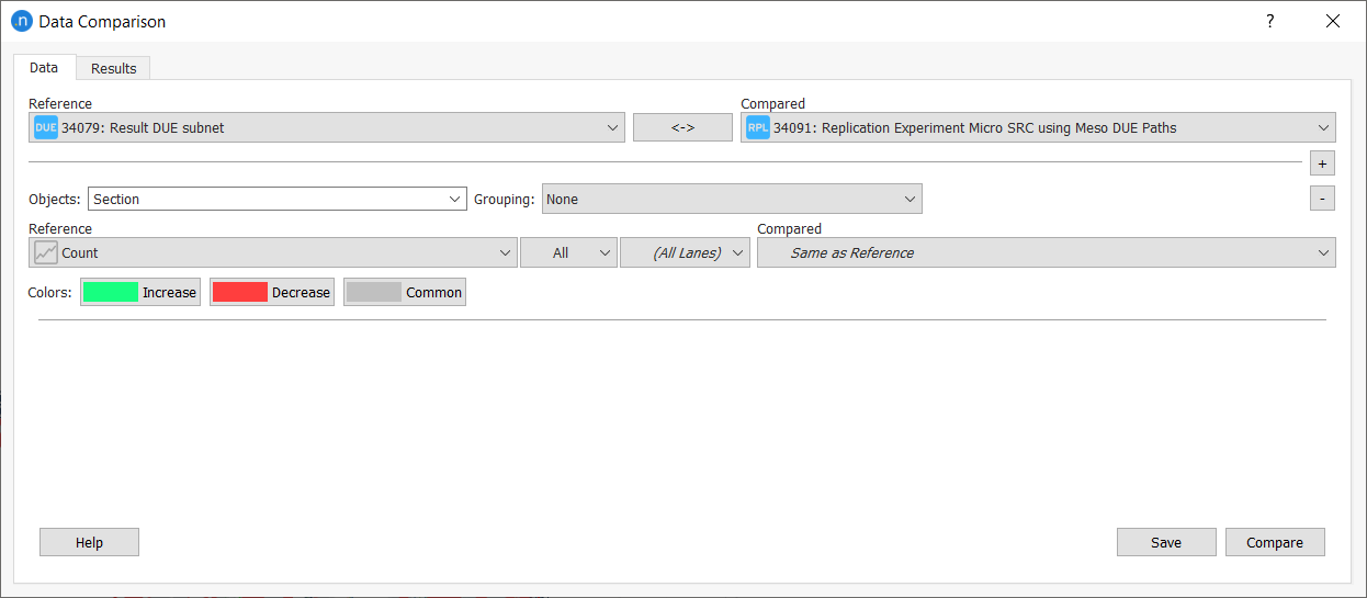
From the Data Analysis menu, select Data Comparison to open its dialog.
From the Reference list, select Result DUE subnet, and from the Compared list, select Replication Experiment Micro SRC using Meso DUE Paths. The screenshot below shows that counts on the road sections are ready to compare.
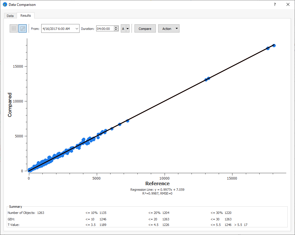
Click Compare to display the results. Click the Graph or Table icons to change the visualization of the data.
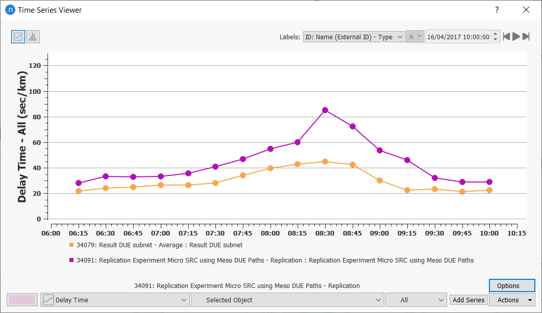
To compare the same outputs in the form of time series, from the Data Analysis menu, select Time Series Viewer to display its dialog.
One at a time, click on the results you want to view in the Subnetworks folder and click Add Series to display the data in the Time Series Viewer. The screenshot below shows a comparison of the average simulated delay time per interval.

Exercise 9. Running a Meso-micro Hybrid SRC Scenario, Loading Dynamic Paths¶

In this exercise, we will run a hybrid simulation that combines a mesoscopic simulation of much of the model with a more detailed microscopic simulation of a critical area where the study focuses on a tram route. First we will create the experiment we need and then define a study area for the microsimulation.

9.1 Creating the experiment¶

Right-click Dynamic Scenario subnet using DUE Paths > New Experiment.
In the Experiment Type dialog select Meso-Micro Hybrid Simulator and Stochastic Route Choice.
Click OK.
Open the experiment and rename it Experiment Hybrid Meso-Micro SRC DTA using Meso DUE Paths.
Set the Using Warm-Up period to 00:15:00 minutes.

9.2 Defining the microsimulation area¶

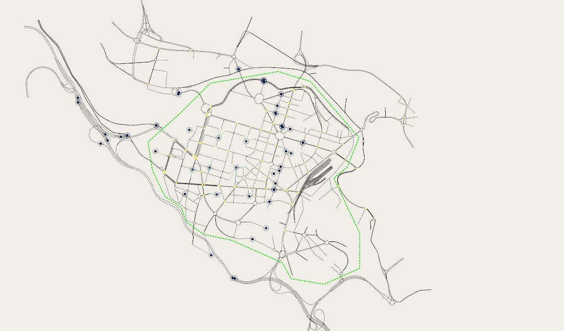
Click and draw a polygon that contains the tram line route: it is marked in green dotted lines below.
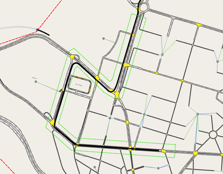
Right-click on the polygon and select Convert to > Simulation Area. A new simulation area object is added to the Simulation Areas folder.
Rename the new object Micro – Simulation Area.
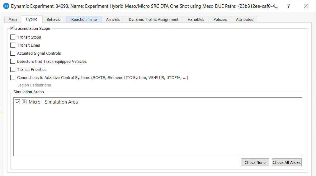
Open Experiment Hybrid Meso-Micro SRC DTA using Meso DUE Paths and click the Hybrid tab. In the Simulation Areas group box, tick Micro – Simulation Area in order to use it in the experiment.
Click the Dynamic Traffic Assignment tab and complete the parameters to match those shown below.
Click OK.
Right-click on the experiment and select New > Replication.
Rename the replication Replication Hybrid Meso-Micro SRC DTA One Shot using Meso DUE Paths.
Right-click on the replication and select Run Batch Simulation. When the replication is complete, the view mode Simulated Flow is selected.
As in Exercise 8.2, use the Data Comparison feature to compare Experiment Hybrid Meso-Micro SRC DTA using Meso DUE Paths and Micro DTA using Meso DUE Paths, showing that there is little difference between the results of each experiment.

We will now compare the speed statistics for a grouping of all the sections inside the microsimulation area.
Right-click on Micro – Simulation Area > Select Objects Inside. The internal sections are now copied and ready to be added to a grouping.
In the Project folder, right-click Data Analysis > New > Grouping Category.
On the Grouping Category Contents dialog, from the drop-down List of Objects of Type, select Section and click OK.
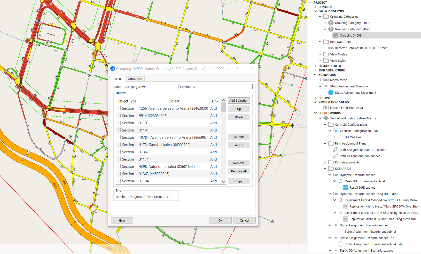
Right-click on the new grouping category, select New > Grouping, and open the new grouping object.
Click Add Selection to fill the dialog with the sections we selected in step 11.
Right-click on the grouping object and select Refresh Statistics for Replication Micro DTA using Meso DUE Paths. Repeat this for Replication Hybrid Meso-Micro SRC DTA using Meso DUE Paths. This will add data to the grouping.
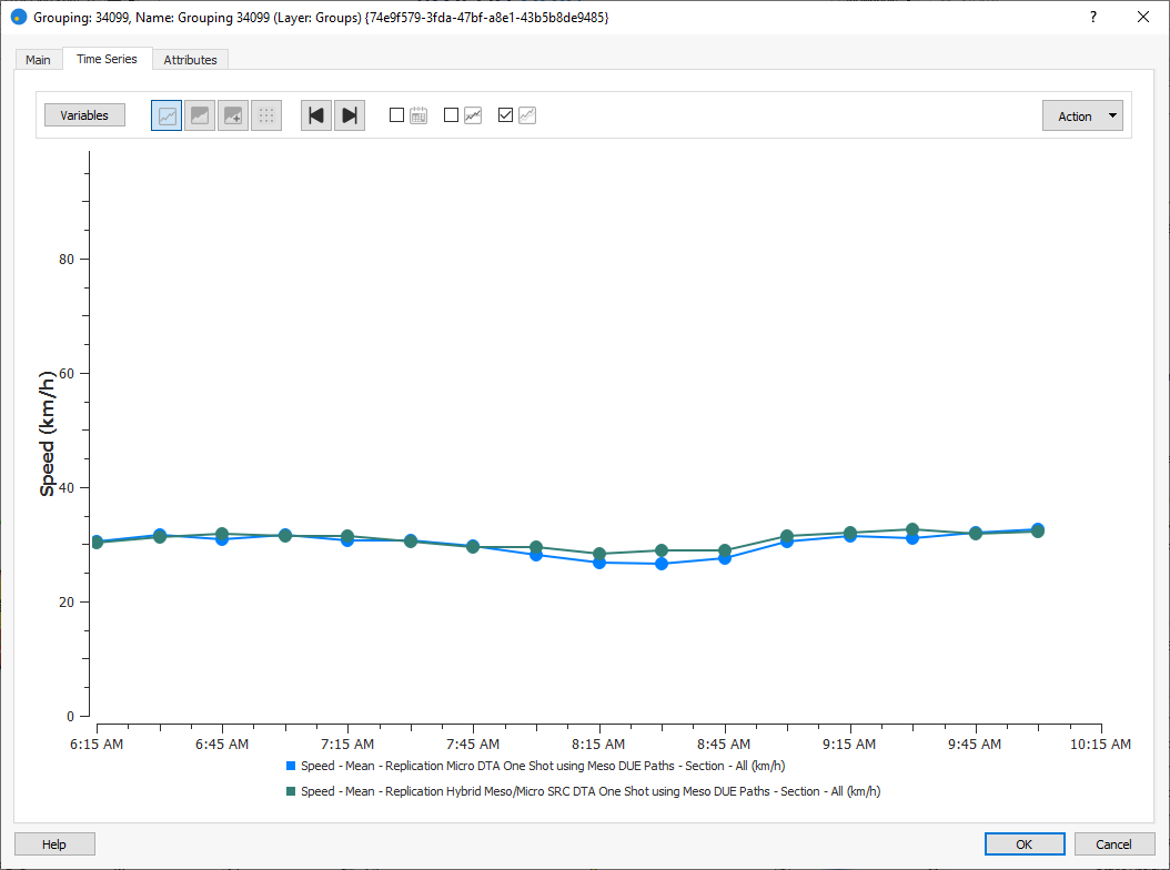
Open the grouping object and click the Time Series tab.
Click Variables and, as we did in the Time Series in Objects exercise in the earlier Microsimulation Outputs tutorials, select metrics to compare the average-speed variables of the two replications (this only applies to the sections in the microsimulation area).

Exercise 10. Running a Macro-meso Hybrid Simulation¶

In this exercise, we will run a hybrid simulation that combines macroscopic and mesoscopic network loading (see Hybrid Macro-Meso Simulator). We will model the city center at a mesoscopic level and the outskirts at a macroscopic level.

The exercise is quite long and is broken down into six stages:

Defining the area and checking costs
Adding a scenario and running the experiment
Changing VDF to BPR
Adding a path assignment plan
Splitting the traffic demand
Running the final experiment.

10.1 Defining the area and checking costs¶

Here we will define the area we want to include in the meso simulation. We will also check to ensure all cost functions use the same units.

Click and draw a polygon that resembles the shape shown in green below.
Right-click on the polygon and select Convert to > Simulation Area.
Rename the new area Meso – Simulation Area.

Now we need to check our cost functions. Route choice is assigned when a vehicle is generated, whether its journey starts in the macroscopic area or the mesoscopic area. The cost of route-choice paths is the sum of all of the volume delay functions (see VDF), turn penalty functions (see TPF), and junction delay functions (see JDF) from the macroscopic area, plus the initial or dynamic cost function from the mesoscopic area.

We must check and ensure that the units across the network are the same (or converted if they are different). This means that all cost functions should give the cost in minutes, for example, rather than a mixture of minutes and seconds.
In the Project folder, click Demand Data > Functions to reveal the list of all functions being used.
For VDF, TPF, and JDF functions, follow steps 6–9.
Double-click each function type to see full details. The example shown in step 7 is the VDF – Example for Motorway.
Click the Usage tab to see if and where the function is used (some might not be in use and will say, for example, 'No section/road type/centroid connection uses this function').
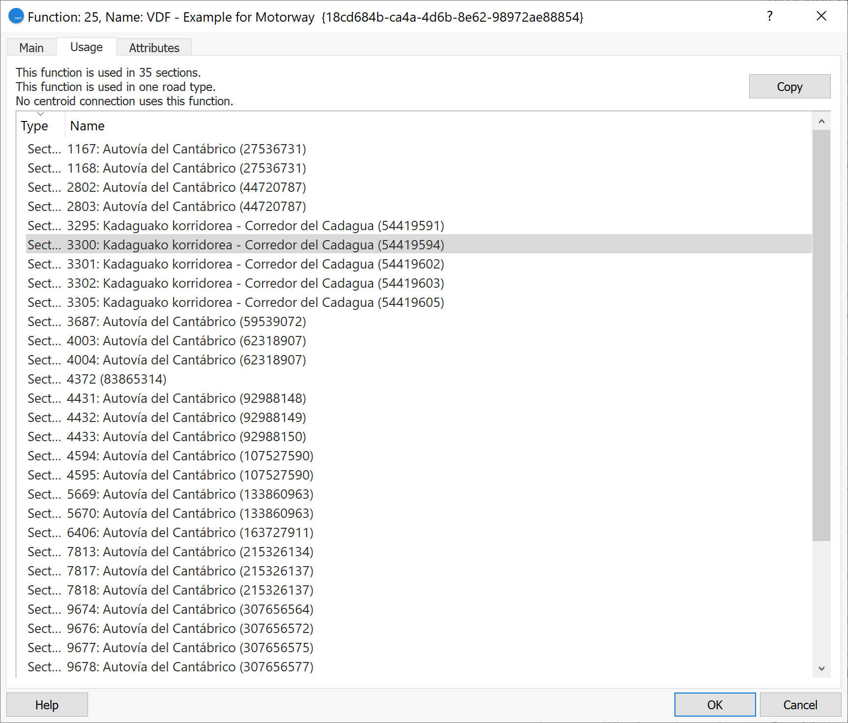
Click the Main tab to see the function code.

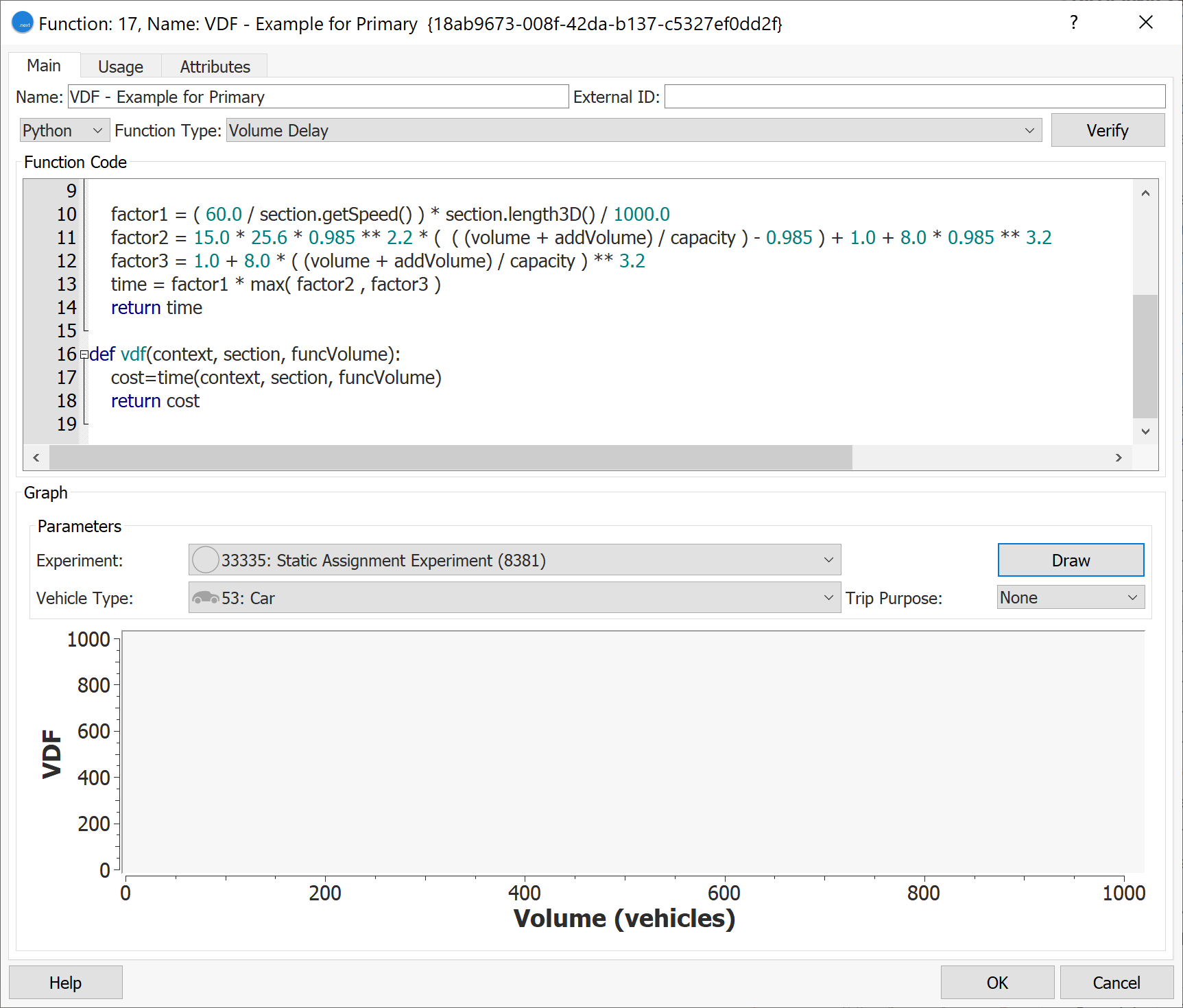
We can see in the code that the cost is the estimated travel time given by the volume function. This is given in minutes by default.
Check and make sure that all costs in all functions being used are also expressed in minutes.

The default cost function for meso (which can’t be accessed from the interface) uses seconds as a unit. We will therefore need to specify the conversion in the scenario’s experiment.

10.2 Adding a scenario and running the experiment¶

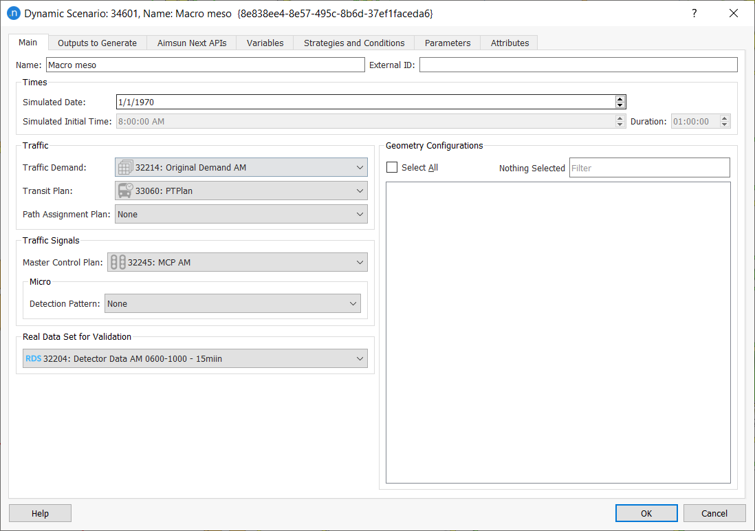
Click Scenario > New > Dynamic Scenario.
Open the new scenario, rename it Macro meso and set the Traffic Demand, Transit Plan, Path Assignment Plan, Master Control Plan, and Real Data Set for Validation as shown below.
Right-click Macro meso > New Experiment. For Network Loading, select Macro-Meso Hybrid Simulator, and for Assignment Approach, select Dynamic User Equilibrium. Click OK.
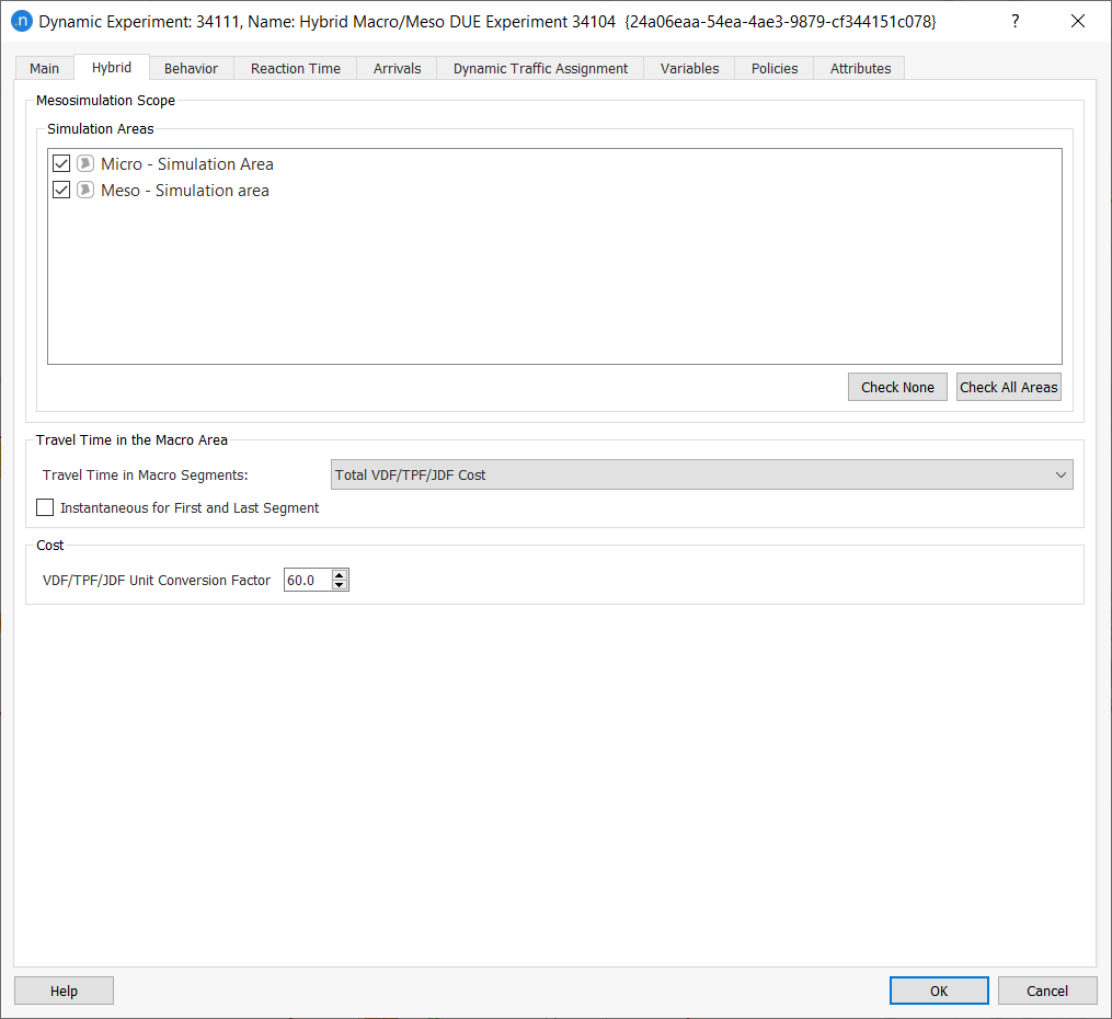
Open the new experiment, rename it Hybrid Macro-Meso DUE Experiment and click the Hybrid tab.
In the Simulation Areas groups box, tick Meso – Simulation Area.
In the Cost group box, leave the VDF Unit Conversion Factor as 60.0. This ensures that all the functions will use minutes for units.
Right-click on the experiment and select New > Result.
Rename the result Result Hybrid Macro-Meso DUE Experiment.
Right-click Result Hybrid Macro-Meso DUE Experiment > Run Batch Simulation.

When the Result dialog is displayed, we can see that convergence is not reached within 20 iterations. This is due to the VDFs used, which are per road type. We should change all VDFs to the BPR function, which is also measured in minutes.

10.3 Changing VDF to BPR¶

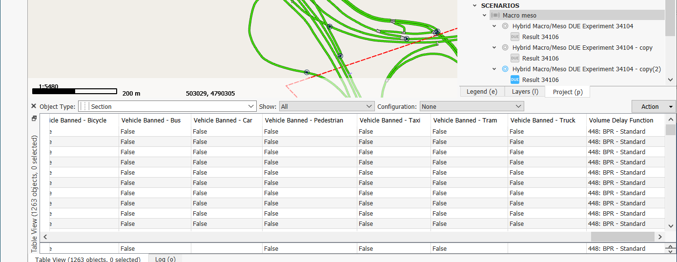
To change the VDFs of all of the sections, you can use the Table view, which sits next to the Log view when displayed.

Click in the 2D view and type 't' to open the Table view. You can also select Window > Windows > Table View. You might find it helpful to click and drag the Table View upwards to see more detail.
In the Object Type list, select Section.
Scroll to the extreme right of the table until you reach the Volume Delay Function column.
At the very bottom of this column, underneath the left–right scrolling bar, there is a cell that affects all the cells above it. In this cell, click and select BPR – Standard to change all VDFs in the column to BPR.

10.4 Adding a path assignment plan¶

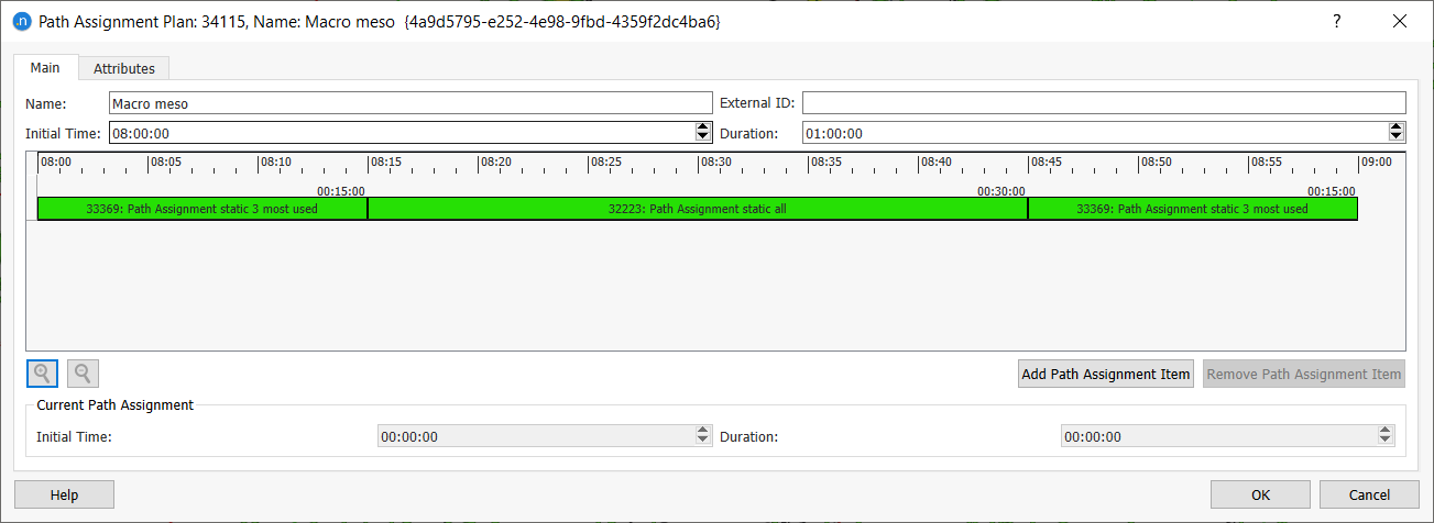
We will now add a path assignment plan using the paths from the static assignment. The path assignment plan will contain two path assignment items. Path Assignment static 3 most used is used twice: at the start and end of the duration:

From 08:00–08:15 – Path Assignment static 3 most used
From 08:15–08:45 – Path Assignment static all
From 08:45–09:00 – Path Assignment static 3 most used.
In the Project folder, right-click Demand Data > New > Path Assignment Plan and rename it Macro meso.
Open the new path assignment plan and click Add Path Assignment Item.
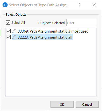
On the Select Objects of Type dialog, tick Path Assignment static 3 most used and Path Assignment static all.
Click OK to add these two paths to the Path Assignment Plan dialog.
Because we are using Path Assignment static 3 most used twice, repeat steps 3 and 4 for this item. All three path assignment items should have been added to the Path Assignment Plan dialog.
Arrange the path assignment items as shown below. You can drag the green bars into place but a more accurate method is to click on a bar and change its Initial Time and Duration values.

10.5 Splitting the traffic demand¶

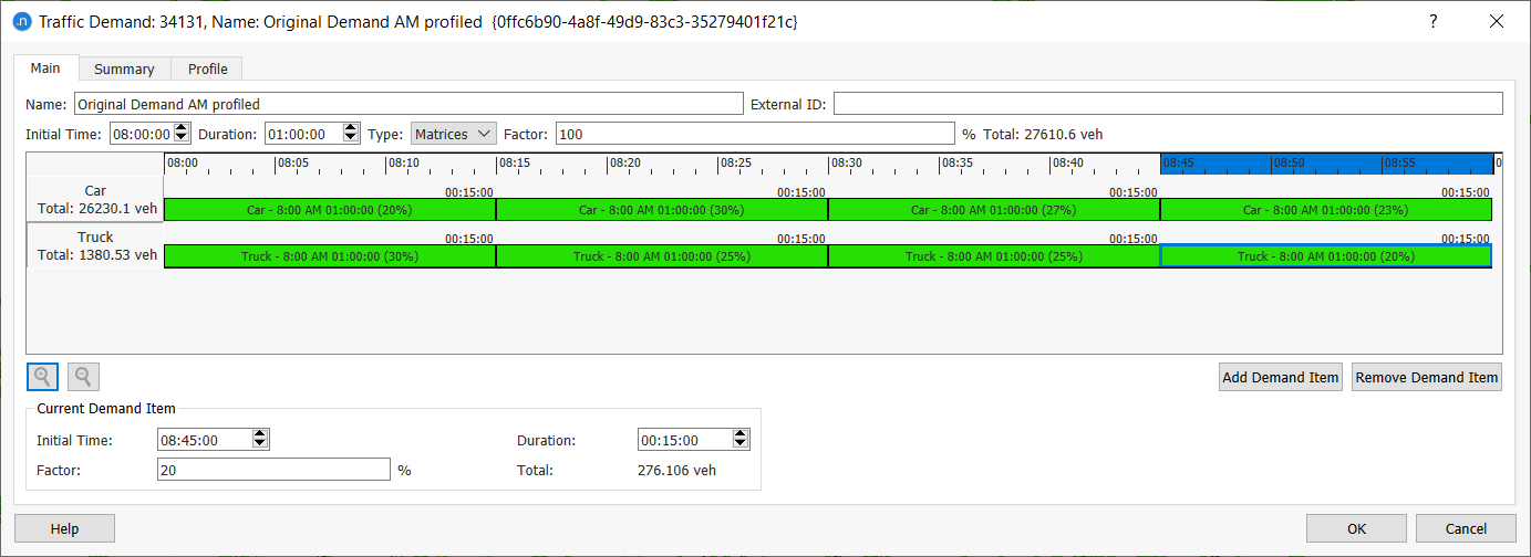
To better represent peak traffic, we will split the traffic demand. We are aiming to split the traffic demand into four OD matrices each for car and truck spread across the one-hour duration. We will give each matrix a percentage factor in line with the following table.

Vehicle Type	08:00–08:15	08:15–08:30	08:30–08:45	08:45–09:00
Car	20%	30%	27%%	23%
Truck	30%	25%	25%	20%

The result will be a traffic demand that resembles the one shown below.

Right-click Original Demand AM > Duplicate. Rename the copy Original Demand AM profiled and open it.
Adjust the existing Car matrix by clicking on its green bar and, below, change Duration to 00:15:00 and Factor to 20 (in line with the table above).
Repeat step 2 for Truck but change its Factor to 30.
Click Add Demand Item.
On the Select Objects of Type dialog, tick both Car and Truck matrices and click OK to add them to the timeline in the Traffic Demand dialog.
Repeat steps 2 and 3 for the new car and truck matrices, ensuring that their Initial Time is 08:15:00, Duration is 00:15:00, and percentage Factor is 30 and 25 respectively, to match the table and screenshot above.
Repeat step 6 for two more sets of car and truck matrices. Their times, duration, and factors can be found in the table above.

10.6 Running the final experiment¶

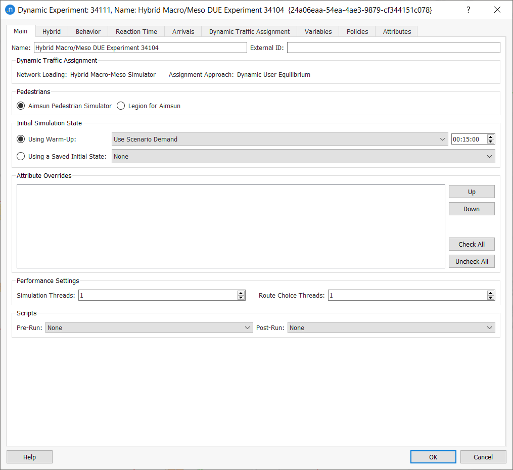
Open Hybrid Macro-Meso DUE Experiment.
On the Main tab, for Using Warm-Up, select Use Scenario Demand from the drop-down list and set the time alongside as 00:15:00.
Click the Dynamic Traffic Assignment tab.
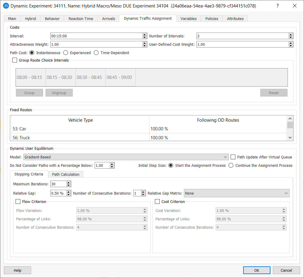
Set the Number of Intervals to 2.
Increase Maximum Iterations to 30.
Right-click Result Hybrid Macro-Meso DUE Experiment > Run Batch Simulation. On completion, we can see that the RGap now converges well.