Cost Functions
The function editor defines several types of functions using the language in Python version 3:
- Basic Cost Functions for the dynamic simulators/Cost Functions for the dynamic simulators using Vehicle Types
- K-Initials Cost Functions for the dynamic simulators
- K-Initials Cost Functions for the dynamic simulators using Vehicle Types
- Route Choice Functions for the dynamic simulators
- Static Macro VDF (Volume Delay Functions)
- Static Macro TPF (Turn Penalty Functions)
- Static Macro JDF (Junction Delay Functions)
- Function Components
- Stochastic Discrete Choice Function
- Adjustment Weight Function
- Transit Waiting Time
- Transit Boarding Function
- Transit Distance Fare Function
- Transit Delay
- Transit Transfer Penalty
- Crowding Discomfort
- Transit Dwell Time
- Distribution Impedance Functions
- Distribution Deterrence Functions
- Distribution Utility Functions
- Modal Split Utility Functions
- Modal Split Discrete Choice Functions
- Car Availability Model Function
- Park and Ride Function
- Dynamic OD Departure Time Rescheduling Arrival Penalty Function
Note: Python version 3 is the default version used by Aimsun Next. Python version 2 still works in Aimsun Next up to and including Aimsun Next 22 but will be discontinued in future releases.
Units 
The default time unit for the macroscopic delay and cost functions in the default templates is minutes. The default unit for the cost functions in dynamic simulations is seconds.
Object Classes
This section makes extensive references to object types, i.e. a GKFunctionCostContext or a DTATurning object. These object types contain methods to get and set the attributes of the object referred to in the function call, e.g.
turn.getAttractiveness(vtype)
returns the modeled attractiveness value for that turn, for a specified vehicle type.
A complete overview of the classes can be found in the Aimsun Next Scripting Documentation and the detail of the methods and the class hierarchy is in the Script Library which refers to the automatically generated web-based reference to the script methods. This web-based documentation should be frequently consulted when writing script functions to determine what data is available for each object class.
Scenario and Experiment Variables
When writing functions, variables can be used to set values of the function parameters. The default value for a variable can be set in the Scenario Editor or varied for an experiment in the Experiment editor. For example, if there is a variable used to control the value returned by a cost function, it is accessed as shown here:
def pbf(context, line, stop):
    res = context.experiment.getValueForVariable( "$COST").toFloat()
    res += line.getBoardingFare()
    return res
where $COST is the name of the variable.
Data used in the functions that are based on trips or centroids can be stored in the Aimsun document as vectors or as matrices to give access to them in the function.
Basic Cost Functions/Cost functions using Vehicle Types
Basic Cost functions allow the user to define, for each link, a generalized cost function not restricted to travel time only. These functions will be used in the Dynamic Route Assignment. They return the cost of a link without distinguishing per vehicle type. Therefore, they cannot make use of variables that have any vehicle type reference, which means all vehicle types will have a common cost.
The Cost functions using vehicle type are the same as the basic cost functions with the only difference that now the vehicle type can be used to distinguish between costs for vehicles.
Signature:
cost( context, manager, section, turn, travelTime) -> double
where:
- context is a GKFunctionCostContext Python object.
- manager is a DTAManager Python object.
- section is a DTASection Python object.
- turn is a DTATurning Python object.
- travelTime is not used.
The context object contains the user class for which the Volume Delay Function is being evaluated. In the case of a basic cost function this object will not be available. In the case of a cost function using vehicle type, the user class will provide the vehicle type for which the function is being evaluated.
The manager object contains the maximum turn attractiveness, attractiveness weight, and user-defined cost weight.
The section object contains among others the section speed, length, and capacity.
The turn object contains the turn origin and destination, its attractiveness, length, and speed.
Basic Example
def cost(context, manager, section, turn, travelTime):
    time = section.getStaTravelT(manager)
    dist = section.length3D()
    w = manager.getAttractivenessWeight()
    aTurn = turn.getAttractiveness()
    aMax = manager.getMaxTurnAttractiveness()
    attract = w * (1 - aTurn/aMax)
    cost = 0.9*time + 0.1*dist + attract
    return cost
Complex Example
In the more complex example, the sectionSpeed and turnSpeed are the minimum between the section or turn speed multiplied by the vehicle speed limit acceptance and the vehicle type maximum desired speed. The cost result (res) takes into account free flow travel times weighted by an attractiveness factor, and is then further modified to add a term for the user-defined cost plus a toll cost based on the section length and the vehicle value of time.
def cost(context, manager, section, turning, travelTime):
    sectionSpeed = min(
        section.getSpeed()*manager.getNetwork().getVehicleById(context.getVehicle().getId()).getSpeedAcceptanceMean(),
        manager.getNetwork().getVehicleById(context.getVehicle().getId()).getMaxSpeedMean())
    turnSpeed = min(
        turning.getSpeed()*manager.getNetwork().getVehicleById(context.getVehicle().getId()).getSpeedAcceptanceMean(),
        manager.getNetwork().getVehicleById(context.getVehicle().getId()).getMaxSpeedMean())
    attractivityFactor = 1+
        manager.getAttractivenessWeight()*
        (1-turning.getAttractiveness()/manager.getMaxTurnAttractiveness())
    res = (section.length3D()/sectionSpeed+ turning.length3D()/turnSpeed)*attractivityFactor
    res = res + manager.getUserDefinedCostWeight()*section.getUserDefinedCost()
    tollPrice = 10      #units in monetary cost per meter taking also into account time units of VoT
    vehicle = context.getVehicle()
    res = res + (section.length3D()+turning.length3D())*tollPrice/vehicle.getValueOfTimeMean()
    return res
K-Initials Cost Functions/K-Initials Cost Functions using Vehicle Types
K-Initials Cost functions allow the user to define, for each link, a generalized cost function not restricted to travel time only. These functions will be used in the Dynamic Route Assignment to calculate the K-Initial Shortest Paths. They return the cost of a link without distinguishing per vehicle type. Therefore, they cannot make use of variables that have any vehicle type reference, so all vehicle types will have a common cost.
The K-Initials Cost Functions Using Vehicle Type are the same as the K-Initials Cost Functions with the only difference that now the vehicle type can be used to distinguish between costs for vehicles.
Signature:
kinicost( context, manager, section, turn, funcVolume ) -> double
where:
- context is a GKFunctionCostContext Python object.
- manager is a DTAManager Python object.
- section is a DTASection Python object.
- turn is a DTATurning Python object.
- funcVolume is the volume to evaluate this function with.
The context object contains the user class for which the Volume Delay Function is being evaluated. In the case of a basic cost function this object will not be available. In the case of a cost function using vehicle type, the user class will provide the vehicle for which the function is being evaluated.
The manager object contains the maximum turn attractiveness, attractiveness weight, and user-defined cost weight.
The section object contains among others the section speed, length, and capacity.
The turn object contains the turn origin and destination, its attractiveness, length, and speed.
The funcVolume object is the volume to evaluate this function with.
Example
def kinicost(context, manager, section, turn, funcVolume):
    dist = section.length3D()
    cost = 10*funcVolume + dist
    return cost
Route Choice Functions
Route Choice functions are defined to be used as a user-defined Route Choice Model. They give the probability for a shortest path.
Signature:
rcf( context, manager, origin, destination, pathsRC, pathsOD, pathsAPA, indexPath ) -> double
where:
- context is a GKFunctionCostContext Python object.
- manager is a DTAManager Python object.
- origin is a DTACentroid Python object.
- destination is a DTACentroid Python object.
- pathsRC is a list of DTAPossiblePath Python objects.
- pathsOD is a list of DTAPossiblePath Python objects.
- pathsAPA is a list of DTAPossiblePath Python objects.
- indexPath is an integer.
The context object contains the user class for which the Route Choice Function is being evaluated and the simulation time.
The manager object contains the maximum turn attractiveness, attractiveness weight, and user-defined cost weight.
The origin object contains variables for the entrances sections and percentages. It represents the origin centroid.
The destination object contains variables for the exit sections and percentages. It represents the destination centroid.
The pathRC is a list with all paths calculated using the route choice for the given destination centroid and origin centroid. It contains DTAPossiblePath objects.
The pathOD is a list with all paths coming from the OD routes. It contains DTAPossiblePath objects. The cost field in the DTAPossiblePath represents the OD percentage defined in the respective OD matrix.
The pathAPA is a list with all paths coming from the Path Assignment results file. It contains DTAPossiblePath objects. The cost field in the DTAPossiblePath represents percentage defined in the Path Assignment results file.
The indexPath represents the path that is being calculated. The range of indexPath is 0 to the sum of the length of pathRC, pathOD, and pathAPA lists.
Example
def rcf( context, manager, origin, destination, pathsRC, pathsOD, pathsAPA, indexPath ):
    prob = 0
    if indexPath==0:
        prob 1
    return prob
It selects always the first route choice calculated path.
Another example that calculates a the probabilities based on a logit selection function:
import math
def rcf( context, manager, origin, destination, pathsRC, pathsOD, pathsAPA, indexPath ):
    scaleFactor = 1;
    allPaths = pathsRC
    numPaths = len(allPaths)
    prob=0
    if indexPath<numPaths:
        aux = 0
        pIP = allPaths[indexPath]
        # pIP is a DTAPossiblePath
        costIP = -pIP.getSPCurrentCost(manager, context.userClass.getDTAVehicleType())/3600.0
        for j in range(numPaths):
            if j!=indexPath:
                pJ = allPaths[j]
                costJ = -pJ.getSPCurrentCost(manager, context.userClass.getDTAVehicleType())/3600.0
                aux = aux + math.exp((costIP-costJ)*scaleFactor)
        prob = 1.0/(1.0+aux)
    print('Prob %d %f'%(indexPath, prob))
    return prob
Static Macro Volume Delay Functions
The Macro VDF (Volume Delay Function) is used to model the travel time or the cost on a section or connection as a function of different parameters such as the volume of the section, its capacity, its length, etc. This type of function is taken into account when doing a static traffic assignment. For more information about VDFs and their role in the assignment, please refer to the Static Traffic Assignment information.
Section modeling
Signature:
vdf( context, section, volume ) -> double
where:
- context, section, and volume are Python objects of the following type: GKFunctionCostContext, CMacroSection, and GKFunctionVolume.
The context object contains the user class for which the Volume Delay Function is being evaluated.
The section object contains the sections parameters that can be used in the static assignment. The parameters that can be consulted are: capacity, length, speed, user-defined costs, additional costs, number of lanes, and user-defined attributes.
The volume object contains the volume for which the Volume Delay Function must be evaluated. Three different volumes can be consulted, total volume, volume per vehicle type and volume per user class. The Volumes are variable values that change during the assignment process.
Function Body:
In the body of the VDF any other arbitrary function that has been defined before the function declaration of the VDF can be used.
Example
def distance(context, section, volume):
    return section.length3D() / 1000.0

def tTime(context, section, volume):
    t0 = 60.0 * distance(context,section,volume) / section.getSpeed()
    c = section.getCapacity()
    v = volume.getVolume()
    t = t0 * ( 1 + 0.15 * (v/c)**4 )
    return t

def vToll(context, section, volume):
    t = 0.15 * distance(context,section,volume)
    return t

def fToll(context, section, volume):
    t = section. getUserDefinedCost()
    return t

def vdf(context, section, volume):
    c1 = 1.0
    c2 = 0.1
    purpose = context.getPurpose()
    if purpose != None:
        if purpose.getName() == "work":
            c2 = 0.15
    c3 = 0.2
    time = tTime(context,section,volume)
    dist = distance(context,section,volume)
    toll = vToll(context,section,volume)
    toll = toll + fToll(context,section,volume)
    cost = c1 * time + c2 * dist + c3 * toll
    return cost
Connection modeling
Signature:
vdf( context, connection, volume ) -> double
where:
- context, connection, and volume are Python objects of the following type: GKFunctionCostContext, CMacroConnection, and GKFunctionVolume.
The context and volume objects are the same as for the Volume Delay Function used for sections. The connection object contains the parameters of the connection that can used during a static assignment. The parameters that can be consulted are: length and user-defined attributes.
Example
def vdf(context, connection, volume):
    length = connection.getLength()
    c1 = 0.05
    return c1 * length
Static Macro Turn Penalty Functions
The Macro TPF (Turn Penalty Function) is used to model the travel time or the cost of a turn as a function of different parameters such as the volume of the turn, its length, etc. This function is taken into account when doing a static traffic assignment. For more information about TPFs and their role in the assignment, please refer to the Static Traffic Assignment information.
Signature:
tpf( context, turn, volume ) -> double
where:
- context, turn, and volume are Python objects of the following type: GKFunctionCostContext, CMacroTurning, and GKFunctionVolume.
The context and volume objects are the same as for the Static Volume Delay Function.
The turn object contains the parameters of the turn that can be used during a static assignment. The parameters that can be consulted include the turn speed, the user-defined costs, the signal timings, and the capacities of the origin section, destination section, and the turn.
Example
def distance(context, turn, volume):
    return turn.length3D() / 1000.0

def tTime(context, turn, volume):
    t = 60.0 * distance(context,turn,volume) / turn.getSpeed()
    return t

def tpf(context, turn, volume):
    c1 = 1.0
    c2 = 0.1
    purpose = context.getPurpose()
    if purpose != None:
        if purpose.getName() == "work":
            c2 = 0.15
    time = tTime(context,turn,volume)
    dist = distance(context,turn,volume)

    cost = c1 * time + c2 * dist
    return cost
Static Macro Junction Delay Functions
The JDF (Junction Delay Function) is used to model the travel time or the cost on a turn as a function of volumes of conflicting turns. This function is used in static traffic assignment. For more information about JDFs and their role in the assignment, please refer to the Static Traffic Assignment information.
Signature:
jdf( context, turn, singleVolume, ownVolume, conflictVolume ) -> double
where:
- context, turn, singleVolume, ownVolume, and conflictVolume are Python objects of the following type: GKFunctionCostContext, CMacroTurning, and GKFunctionVolume.
context and turn are identical to the context and turn of the TPF.
singleVolume is the volume passing through the turn.
ownVolume is the total volume of all the turns that share an origin lane with the turn.
conflictVolume is the total volume of turns that geometrically conflict with the turn (automatic option) or the volume of turns specified by the user in the Conflict Turns table in the Node editor.
Example
def jdf(context, turn, singleVolume, ownVolume, conflictVolume):
    volume = singleVolume.getVolume()
    conflict = conflictVolume.getVolume()
    ratio = 0.0
    if ( volume != 0.0):
        ratio = conflict / volume
    delay = 0.2 * ratio
    return delay
Cost Function Errors and Constraints
The functions TPF, JDF, and VDF are subject to certain constraints which will trigger errors and the cancellation of dynamic simulations, static assignments, and static adjustments.
These constraints are as follows.
- a turn cost (sum of TPF + JDF) must be > = 0
- a section cost (VDF) must be > 0
- a unidirectional centroid connector (VDF) must be > = 0
- a bidirectional centroid connector (VDF) must be > 0
- a supernode trajectory cost (sum of TPF + JDF) must be > 0
If costs do not meet these constraints, affected processes will be cancelled and error messages displayed in the Log window.
Function Components
Function Components are used to obtain extra outputs from Static Assignments or Dynamic Traffic Simulations for Sections, Connections, and Turns and also for Path statistics.
If the definition of a VDF, TPF, JDF, DCF, ICF contains a subfunction as part of its calculation then this subfunction can be declared as a Function Component and its output displayed in the statistics of the object the function is assigned to. Additionally, path statistics for each component will also be calculated.
For example, if a JDF was defined as:
    def jdf(context, turning, singleVolume, ownVolume, conflictVolume):
    jdattribute = calculateJDFAttr( context, turning, singleVolume, ownVolume, conflictVolume)
    delay = computation
    return delay

    def calculateJDFAttr(context, turning, singleVolume, ownVolume, conflictVolume):
    attr = computation
    return attr
where function calculateJDFAttr() computes one part of the turn junction delay, then that subfunction can be declared as a Function Component, identifying it by the name 'calculateJDFAttr'.
Example for a DCF:
    def distanceInKm(context, manager, section, turn, travelTime):
        return section.length3D()/1000.0+turn.length3D()/1000.0

    def cost(context, manager, section, turn, travelTime):
        turncost = turn.getStaTravelT(manager)+manager.getUserDefinedCostWeight()*section.getUserDefinedCost()
        return turncost
Note that the main function does not necessarily call the subfunction.
In the Function Component editor, the Function String must match exactly with the name of the corresponding subfunction and the Name will be used as the name for the new column that will be generated.
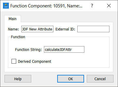
The code corresponding to the subfunction will be evaluated separately and a new column for the object will be created containing the values it computes. As the Function Component is called separately, the subfunction must have exactly the same arguments as the main function in order to be correctly evaluated.
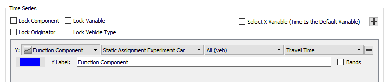
The Function Component can be viewed in the timeseries of a simulation object as shown below or their aggregated values for paths and OD matrices (weighted by number of vehicles on each path) in the Path Assignment folder.
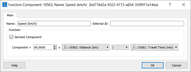
Derived Function Components can also be declared and they are computed as the combination of other components. For example, if a travel time component and a distance component exist, the speed can be computed without declaring a speed function in the VDF, TPF or JDF, but as a combination of the existing components, as shown in the image below. In terms of aggregated data for the path, using Derived Function Component implies an important computation difference: defining the speed as a derived component will give the path mean speed (distance of the path divided by travel time of the path, once these two values have been calculated), whereas defining speed through subfunctions as a non-derived function component would total the speeds through the path to compute the path value for this column.
In case of an invalid value as input in a Derived Function for an interval, the Time Serie shows NaN. Idem for a zero-division. If all intervals are invalid, the derived function is not included.
Stochastic Discrete Choice Functions
The Stochastic Discrete Choice function is used to calculate the probabilities each path is being used. This function is taken into account when doing a Stochastic Traffic Assignment. For more information about SDCs and their role in the assignment, please refer to the Static Traffic Assignment information.
Signature:
sdc( context, pathChoice ) -> double
where:
- context and pathChoice are Python objects of the following type: GKFunctionCostContext and GKPathChoice.
context is identical to the context of the VDF. pathChoice is a set of paths and their costs.
Example
def sdc(context, pathChoice):
    mu = 100
    total = 0.0
    cost = 0.0
    res = []
    for pathCost in pathChoice.getCosts():
        total += math.exp( mu * 1.0/pathCost )
    for pathCost in pathChoice.getCosts():
        res.append( math.exp(mu * 1.0/pathCost) / total )
    return res
Adjustment Weight Functions
The Adjustment Weight function is used to give different (not fixed) weights to the counts (to the difference between counts and assigned volumes) in the adjustment process. It returns a value that multiplies the Reliabilities previously set by the user (1 by default). This function is taken into account when doing an OD Adjustment. This function is applied to values from the detector data for sections, detectors, and turns but not for the Exit/Entrances additional comparison values for which Reliabilities can be set in the Centroids and Sections tab.
Signature:
adw( context, observed ) -> double
where:
- observed is a double.
observed is the value in the Time Series used in the Adjustment, the count that has to be compared with the assigned volume.
Example
def adw( context, observed):
    res = 1.0
    if observed > 0.0:
        res = 1.0/math.pow(observed,0.5)
    else:
        res = 0.0
    return res
Transit Waiting Time Functions
The Transit Waiting Time function is used to model the waiting time at a Transit Stop until boarding a vehicle. This function is used when undertaking a Transit Assignment.
Signature:
pwf( context, interval ) -> double
where:
- context is a Python object of type GKFunctionCostContext and interval is a double.
context gives the experiment context and interval is the combined mean headway between transit vehicle arrivals of the possible boarding lines.
Example
def pwf( context, interval ):
    frequency = 60.0 / interval
    res = 20.0 * math.exp(-0.3 * frequency)
    return res
Transit Boarding Functions
The Transit Boarding function is used to model the cost of boarding a transit vehicle at a Transit Stop, that is, the access fare. This function is used when undertaking a Transit Assignment.
Signature:
pbf( context, line, stop ) -> double
where:
- context, line, and stop are Python objects of the following type: GKFunctionCostContext, PTLine, and PTStop.
context gives the experiment context. line is the Transit Line the passenger wants to board to. stop is the stop at which the passenger is waiting to board.
Example
def pbf(context, line, stop):
    res = line.getBoardingFare()
    return res
Transit Distance Fare Functions
The Transit Distance Fare function is used to model the distance/in-vehicle fare in a Transit trip on a Transit Line. This function is used when undertaking a Transit Assignment.
Signature:
pff( context, line, ptsection ) -> double
where:
- context, line, and ptsection are Python objects of the following type: GKFunctionCostContext, PTLine, and PTSection.
context gives the experiment context. line is the Transit Line the passenger wants to board to. ptsection is the set of segments/sections from one Transit Stop to the next one being evaluated.
Example
def pff( context, line, ptsection ):
    distance = ptsection.getDistance()/1000.0
    fare = line.getDistanceFare()
    res = distance * fare
    return res
Transit Delay Functions
The Transit Delay function is used to model the travel time or the cost on a Transit segment on a Transit Line using the in-vehicle time. This function is used when undertaking a Transit Assignment.
Signature:
pdf( context, line, ptsection ) -> double
where:
- context, line, and ptsection are Python objects of the following type: GKFunctionCostContext, PTLine, and PTSection.
context gives the experiment context. line is the Transit Line. ptsection is the set of segments/sections from one Transit Stop to the next one being evaluated.
Example
The default delay function, applied where there is no user-defined function, is:
def pdf( context, line, ptsection ):
    distance = ptsection.getDistance() / 1000.0
    # Constant speed 20 km/h
    speed = 20.0 / 60.0
    delay = distance / speed
    # Return value in minutes
    return delay
Transit Transfer Penalty Functions
The Transit Transfer Penalty function is used to model the penalty for transfers from line to line during a transit trip. This function is used when undertaking a Transit Assignment and it is selected at the Experiment editor. Usually people avoid transfers in transit because of the inconvenience they produce, therefore, this function will penalize the decision to make a transfer.
Signature:
ptp( context ) -> double
where:
- context is a Python object of type GKFunctionCostContext and gives the experiment context.
Example
def ptp( context ):
    res = 7.0
    # minutes
    return res
Crowding Discomfort Functions
The Crowding Discomfort function is a non-decreasing function used to model the discomfort generated by sharing a limited space while using transit with other passengers. This function is used when undertaking a Transit Assignment and it is selected at the Transit Line editor.
Signature:
pcd( context, line, volume ) -> double
where:
- context is a Python object of the type GKFunctionCostContext that gives the experiment context.
- line is a Python object of the type PTLine that gives the Transit Line.
- volume is a double that gives the volume that travels from one Transit Stop to other Transit Stop using the Transit Line line.
Example
def pcd( context, line, volume ):
    initialDiscomfort = 1
    seatingCapacity = line.getSeatingCapacity()
    alfa = 6
    beta = 1
    loadFactor = volume/seatingCapacity

    if volume > 0:
        discomfort = initialDiscomfort + (1 - (seatingCapacity/volume)) *initialDiscomfort*beta*math.exp( alfa * (loadFactor-1) )
    else:
        discomfort = initialDiscomfort

    if discomfort < p:
        discomfort = initialDiscomfort

    return discomfort
Transit Dwell Time Functions
The Transit Dwell Time function is used to model the dwell time of transit vehicles at stops, taking the volume of passengers boarding and alighting during the assignment into account. Use this function when undertaking a static Transit Assignment.
Signature:
pdt( context, line, ptstop, alightingVolume, boardingVolume ) -> double
where:
- context is a Python object of the type GKFunctionCostContext that gives the experiment context.
- line is a Python object of the type PTLine that gives the Transit Line.
- ptstop is a Python object of the type PTStop that gives the Transit Stop.
- alightingVolume gives the aggregated volume of passengers alighting at the transit stop from the transit line for the whole assignment period.
- boardingVolume gives the aggregated volume of passengers boarding at the transit stop from the transit line for the whole assignment period.
Example
Note: Coefficients must be modified accordingly
def pdt( context, line, ptstop, alightingVolume, boardingVolume ):

    defaultDuration = 0.5

    dwellAlighting = 0.01

    dwellBoarding = 0.05

    dwell = defaultDuration + dwellAlighting*(alightingVolume/line.getNbRuns()) + dwellBoarding*(boardingVolume/line.getNbRuns())

    return dwell
Distribution Impedance Functions
The Distribution Impedance function calculates the combined impedance of the available modes. This function is executed within the Distribution process and it is selected in the Distribution and Modal Split Area.
Signature:
dif( context, origin, destination, modes, data ) -> double
where:
- context (GKFunctionCostContext) gives the experiment context.
- origin (GKCentroid) is the origin centroid.
- destination (GKCentroid) is the destination centroid.
- modes (vector of GKTransportationMode) are the modes are available and combinable for the combined impedance calculation.
- data (SkimDataProvider) gives access to the skim and parking values.
Example
\# Distribution Impedance Function
from PyLandUsePlugin import *

def dif( context, origin, destination, modes, data ):
    cost = 0.0
    for mode in modes:
        cost += data.getSkimValue( SkimType.eCost, mode, origin, destination )
    return cost / len( modes )
Distribution Deterrence Functions
The Distribution Deterrence function calculates the interactivity of centroid as a function of the impedance. This function is executed within the Gravity Model Distribution process and can be set in the Gravity Model Distribution Experiment.
Signature:
ddf( context, cost ) -> double
where:
- context (GKFunctionCostContext) gives the experiment context.
- cost (double) is the cost or impedance.
Example
\# Distribution Deterrence Function

def ddf( context, cost ):
    return 1.0 / cost
Distribution Utility Functions
The Distribution Utility function calculates the utility of all trip options from an origin or to a destination. This function is executed within the Destination Choice Distribution process and can be set in the Destination Distribution Experiment.
Signature:
duf( context, data, modes, centroid, centroids ) -> double
where:
- context (GKFunctionCostContext) gives the experiment context.
- data (SkimDataProvider) gives access to skim matrices.
- modes (vector of GKTransportationMode) are the modes available and combinable for the utility calculation.
- centroid (GKCentroid) is the origin or destination centroid under consideration.
- centroids (vector of GKCentroid) are the centroids available from the centroid under consideration.
Example
\# Distribution Utility Function
from PyLandUsePlugin import *

def duf( context,data,modes,centroid, centroids):
    uts = []
    c1 = -1.0
    for i in range(len(centroids)):
        res = 0.0
        for mode in modes:
            res += c1 * data.getSkimValue( SkimType.eCost, mode, centroid, centroids[i] )
        uts.append(res)
    return uts
Modal Split Utility Functions
The Modal Split Utility function calculates the utility value per transportation mode for each OD pair. This function is executed within the Modal Split process and is selected in the Distribution and Modal Split Area.
Signature:
def msu( context, origin, destination, mode, data ): -> double
where:
context: An instance of a GKFunctionCostContext, gives the experiment context. origin: An instance of a GKCentroid, the origin centroid. destination: An instance of a GKCentroid, the destination centroid. mode: The transportation mode. data: An instance of a SkimDataProvider, gives access to the skim and parking values.
Example
\# Modal split utility function
from PyLandUsePlugin import *

def msu( context, origin, destination, mode, data ):
    c1 = -1.0
    c2 = -1.5
    res = c1 * data.getSkimValue( SkimType.eCost, mode, origin, destination )
    res += c2 * data.getSkimValue( SkimType.eDistance, mode, origin, destination )
    return res
Modal Split Discrete Choice Functions
The Modal Split Discrete Choice function calculates the probability for each mode of choice as a function of the utility. This function is executed within the Modal Split process and can be set in the Modal Split Experiment.
Signature:
def mcf( context, vehicles, utilities ):
where:
context (GKFunctionCostContext) gives the experiment context. vehicles (vector of GKVehicle) are the vehicles belonging to the corresponding available transportation modes. utilities (vector of double) gives the utility values for each mode (vehicle).
Example
\# Modal Split Discrete Choice Function
from math import exp
from PyLandUsePlugin import *

def mcf( context, vehicles, utilities ):
    res = []
    total = 0.0
    for utility in utilities:
        if utility!=0:
            total = total + exp( utility )

    for i in range( 0, len(modes) ):
        if utilities[i]!=0:
            res.append( exp( utilities[i ] ) / total )
        else:
            res.append( 0.0 )
    return res
Car Availability Model
The Car Availability Model function is used to calculate automatically the Car Availability and Non Car Availability percentages per zone for the Generation/Attraction procedure.
Signature:
cam( centroidData, purpose, modelConnection ) -> double
where:
- centroidData, purpose, and modelConnection are Python objects of the following type: CentroidGenerationAttractionData, GKTripPurpose, and GKModelConnection.
centroidData gives access to the Car Availability data (Average Household Size and Car Ownership (per 1000 inhab)) . purpose is the Trip Purpose being evaluated, which contains some Car Availability related parameters. modelConnection gives the information needed to determine network overrides that apply.
Example
def cam( centroidData, purpose, modelConnection ):
    carAvailability = 100.0
    return carAvailability
Park and Ride Function
The Park and Ride Traffic Action changes the destination centroid of a vehicle in response to congestion. The vehicle can choose to travel to a different centroid from where the traveler will proceed by transit. The Park and Ride function returns the overall perceived cost of using transit and can take into account the vehicle's value of time and the relative perceptions of the time of travel in a car and on a bus and the cost of parking. See the Park and Ride Centroid's attributes for information about setting the park and ride function, and the park and ride centroid's price and capacity, that can be used as an input for the Park and Ride function.
Signature:
def par( context, manager, centroid, vot, travelTime, travelTimePT )
where:
- context is a GKFunctionCostContext Python object.
- manager is a DTAManager Python object.
- centroid is the park and ride centroid, a DTACentroid Python object.
- vot is the vehicle's Value of Time
- traveltime is the expected time of the trip in current circumstances (from the section where the park and ride is evaluated to the original destination).
- traveltimePT is the expected time of the trip using Transit (from the park and ride to the original destination in Transit).
Example
def par ( context, manager, centroid, vot, travelTime, travelTimePT )
    cost = TravelTimePT + 1.5 * centroid.getDataValueDoubleByID( centroid.parkAndRidePriceAtt )
    return cost
Dynamic OD Departure Time Rescheduling Arrival Penalty Function
The penalty functions implement the scheduling cost of arriving early or late. This is the extra cost to be added to the travel cost as a result of arriving early or late, the adjustment process then minimizes the overall costs for all travelers.
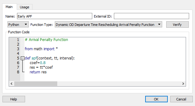
To create a schedule cost function, use the function editor to edit a new function and label it as a Dynamic OD Departure Time Rescheduling Arrival Penalty Function. The default function is a merge of a linear and an exponential function to progressively penalize higher arrival time discrepancies. The function parameters are:
- context A GKFunctionCostContext object
- tt: The difference in arrival time between the preferred arrival time window and the actual time. i.e. the number of seconds early or late.
- interval The length of an arrival or departure time window.
The function should be programmed to use different parameters for each vehicle class or user class as the cost of being late will vary according to trip purpose and time of day. The user class is available in the context parameter for the function.
Function Dialog
Double-click on a function to open its dialog box. In the Function dialog you can:
- Rename a function
- Change its Function Type from a drop-down list of available functions (e.g. Cost, Cost Using Vehicle Type, Route Choice, and many more)
- Refine the code of the function by typing directly into the Function Code box
- To check the validity of the code, click Verify. You will be notified that the code is correct or presented with details of any errors.
-
Draw a graph of the function.
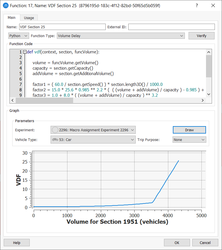
Drawing a Graph
As you can see from the previous screenshot, in the lower half of the Function dialog you can draw a graph of the function as it applies to an object in the network.
To draw a function graph:
-
Select from the following parameters' drop-down lists.
-
Experiment (an available experiment)
-
Vehicle Type
-
Trip Purpose (if available, 'None' if not).
-
-
In the active 2D view, click an object that corresponds to the type of function (e.g. click a section for a VDF).
-
Click Draw to display the graph.
Usage Tab
The Usage tab lists all the objects in the network that use the function.
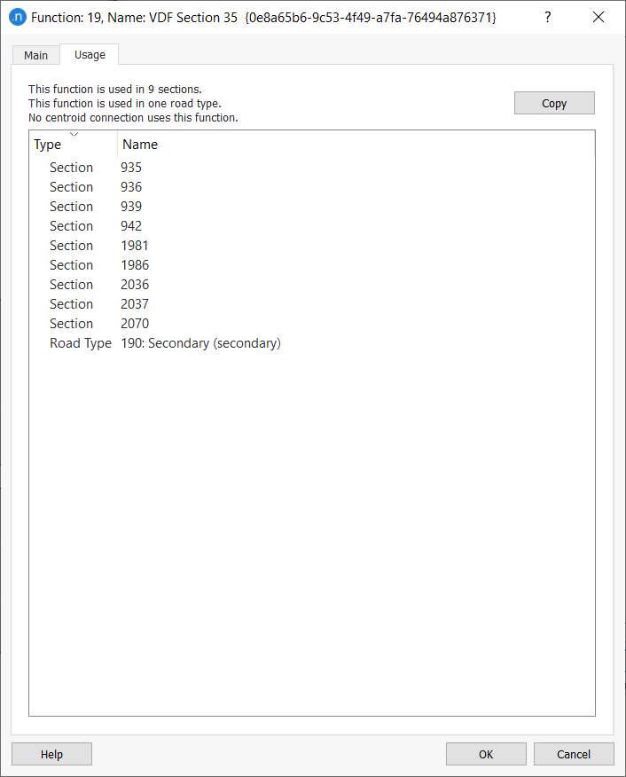
-
Click on a listed object to highlight it in the 2D view.
-
Double-click an object to open its dialog to inspect or change its parameters.