Understanding the Elasticities in an OD Adjustment

The weights in both Static and Dynamic OD Adjustment processes control how important role play each of the components of the objective function in the iterative process. For the OD term the weight is defined through the user-defined elasticity value. The aim of the adjustment process is to minimize the following objective function after every iteration.

These components measure the Goodness-of-Fit (GoF):

• \(γ_{1}\frac12(G-\hat{G})^2\) refers to the difference between the current adjusted OD matrix and the seed OD matrix, where:
  • \(γ_{1}\): weight factor with respect to the traffic demand (OD matrices)
  • \(G\): adjusted OD matrix
  • \(\hat{G}\): seed OD matrix
    
• \(γ_{2}\frac12(V(G)-\hat{V})^2\) refers to the difference between the current adjusted volumes and the observed measurements, where:
  • \(γ_{2}\): weight factor for the observed measurements with a range between 0 and 1
  • \(V(G)\): adjusted volumes updated after every iteration
  • \(\hat{V}\): observed measurements read from Real Data Set
    
• \(γ_{3}\frac12(P-\hat{P})^2\) refers to the difference of the current adjusted and the base trip length distribution resulted from the first iteration (available only in static OD Adjustment)
  • \(γ_{3}\): weight factor for the trp length distribution
  • \(P\): updated trip length for OD trips splitted per 1-km cells calculated in every iteration
  • \(\hat{P}\): trip length for OD trips splitted per 1-km cells in the first iteration

Figure 1 shows that in both Dynamic (left window) and Static (right window) OD Adjustment experiment tabs, the user can set the demand elasticity (\(e_{1}\)) per User Class. The trip length distribution elasticity (\(e_{3}\)) can be set only in static OD Adjustment per User Class. Once set, then both Demand and Trip Length Distribution elasticities are translated into weights (\(γ_{1}\)) and (\(γ_{3}\)) using the following formula: \(γ_{a}= \frac{1}{e_{a}}-1\)

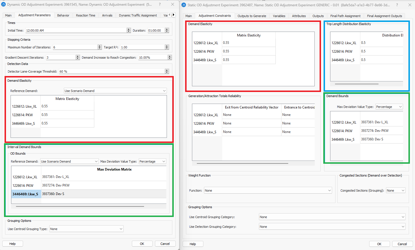
That \(γ_{1}\), \(γ_{2}\), \(γ_{3}\) are the weighting factors reflecting the uncertainty of the information contained in the Seed OD matrix, observed counts and observed TLD, respectively.

The value for the weight \(γ_{2}\) is taken by the Real Data Set if this includes a value per measurement named Reliability. This value is considered in the adjustment process as a weight for the difference between observed and assigned data. The larger the Reliability, the higher the importance of this error term to the overall objective function. The reliability can take values between 0 and 1.

In detail:

By the default the weight value \(γ_{2}\) is set to 1.0. However, the weight depends on the following conditions:

• Reliability: if the RDS has a reliability column, it multiplies the weight by the value in the reliability column.
• Weight Function (only in Static OD Adjustment): it multiplies the weight by the value obtained from evaluating the Weight Function.
• Detectior Coverage (only Detectors & Detector Stations): The number of lanes of the section covered by the detector/station / number of lanes (similarly for turnings). It multuplies the weight by this value. Always applied. I don’t know why is it applied in this way. Maybe to favour detectors which have total coverage of the section.

So, the weight may result by the following calculation:

\(weight = 1.0 * Reliability * WeightFunction * DetectorCoverage\)

While the elasticities are measures of how firmly anchored the adjusted matrix is to the prior matrix, other conditions can then constrain the adjusted value, such as the Demand Bounds, which is specified through a matrix of constraints per cell and per User Class.

If the prior OD matrix for one user class is well established and known to be accurate, then a demand elasticity close to zero would be appropriate as the structure of the initial OD matrix is preserved. Conversely, if the prior matrix is less accurate – perhaps derived from an older model or where there were known to be subsequent land-use changes – then the matrix would be expected to change more significantly in the adjustment scenario. Therefore a demand elasticity value (\(e_{1}\)) closer to 1 would be appropriate.

Similarly the user should set the values in the trip length distribution elasticity. However, in most of the cases, the result of this difference \((P-\hat{P})^2\) ends up to a very low values as it refers to a difference between tow percentages. To influence the OD adjustment process, the elasticity values should be very low values.

The elasticity values cannot be predefined as the vectors and parameters in the objective function depend on many indicators such as the size of the network, the type of the network (urban interurban, mixed), the number of ODs, the size of the traffic demand, the number of detectors, the reliability of the data, the magnitude of the detector data etc. Subsequently, the values defined in one project may not reach the same outcome in another project. Our recommendation is to start with some values and run several tests to understand the impact of each elasticity in the process and then fine-tune each elasticity value.

Following you can find examples testing a range of values for elasticities that may help you understand the impact of the elasticities in the adjustment process. Note that some of these values are not realistic but were set to show the limits of the adjustment process. For instance:

• When elasticity is set to 0.01, then the weight is equal to 99 for the OD term, that means that there is a huge confidence in the initial OD matrix
• When the weight is equal to 1 for the count term, we trust much less the observed counts

We need to consider values for the weights (i.e. elasticity) in the OD term in relation to how well the initial matrix can reproduce the observed counts (RDS). So if weight for counts is always 1, then the elasticity values should vary between 0.5-1, otherwise we make the assumption that we trust more the initial matrix than the RDS.

Demand Elasticity

The elasticity values for the demand control how much the values in the adjusted matrix can vary in the adjustment procedure.

It can be understood as the strength of the reactive force that opposes to the changes of the demand with respect to the reference demand.

An elasticity value closer to zero results in high weight for the OD term in the objective function, hence, the deviation from the seed demand is small. When elasticity is 1, the weighting factor is 0 (reference to the equation), which means that the OD term is not considered in the objective function. Removing this term gives flexibility to the algorithm to search in a wider space of solutions, instead of restricting the deviation Elasticity value 1 can be selected in cases where the quality of the seed OD matrix is not good.

That means, the closer to 0 the stronger this reaction is to any deviation from the original demand whereas the closer to 1, the weaker it is. In the corner case where it is 0, there is no reaction to a change from the original demand. 

Example

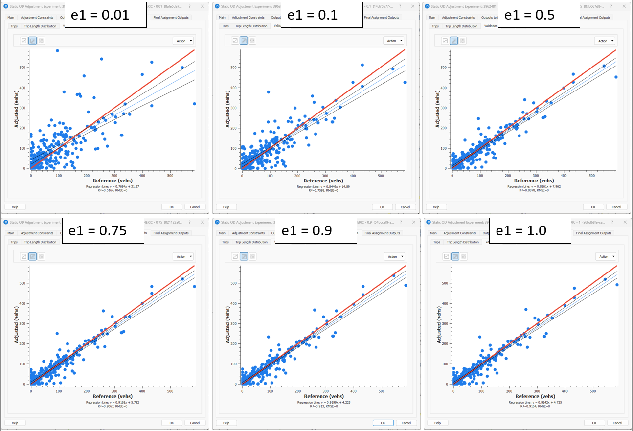
In a sample network, while keeping all the rest of the input parameters fixed, we tested the following 6 values of demand elasticities:

\(e_{1}\) = {0.01, 0.1, 0.5, 0.75, 0.9, 1.0}

To translate those elasticities into a weight (\(γ_{1}\)) used in the objective function, we apply the formula: \(γ_{1}= \frac{1}{e_{1}}-1\). 

\(γ_{1}\)= {99, 9, 1, 4, 0.111, 0}

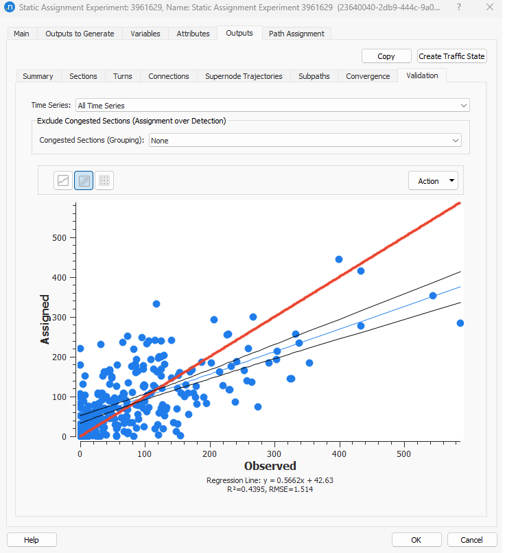
The result of the static assignment before the adjustment:

What we expect to undestand from this experiment is that when using an elasticity close to 0 (high weight), we restrict the adjustment of the OD trips of the seed matrix. So, the process does not allow the cells to significantly change along the iterations, to modify (adjust) the demand and therefore to improve the validation. As a consequence of this restriction, it is expected that the Trip Length Distribution will not change when comparing the final adjustment result to the result of the first iteration of the adjustment. In contrast, when using a demand elasticity close to 1 (low weight), then we give freedom to the cells in the seed OD matrix to move the OD trips so that the validation improves. In this case, the Trip Length Distribution will change significantly as the trips

After running those experiments, the OD Adjustment came out with the following results:

Validation tab

Setting small demand elasticity values (i.e.: 0.01), the validation between adjusted and reference volumes did not improve as the OD Trips were not modified sufficiently whereas when setting the demand elasticity close to 1 (i.e.: 0.9), the validation R2 and Slope improved.

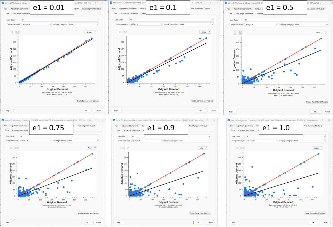
Trips tab

Setting small demand elasticity values, the OD trips did not modified sufficiently while when demand elasticity value was set close to 1, it was given more freedom in the adjustment process to modify the OD trips in the seed matrix.

Trip Length Tab

When the demand elasticity is set close to 0, the Trip Length Distribution does not change as the trips remain almost same.

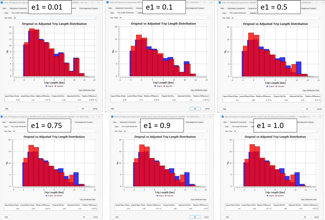
The conclusion is that the closer to 1 the demand elasticity value is set, the more freedom is given to the cells in the seed matrix to adjust, so that it improves the validation criteria (R2, Slope).

Again, these are just examples where the elasticity values tested were randomly chosen, so do not take those elasticity values as the default values for your project.

Trip Length Distribution Elasticity

The Trip Length Distribution Elasticity is only defined in the Static OD Adjustment Experiment.

The same concept of elasticity as in the demand elasticity is also available for the Trip Length Distribution. However in this case, instead of comparing the reference and adjusted demands, the comparison is between the bins of the original trip length distribution calculated after the first iteration and the bins of the final iteration. Where bins are the OD trips aggregated in cells of 1-km ranges (0-1, 1-2, 2-3...13-14).

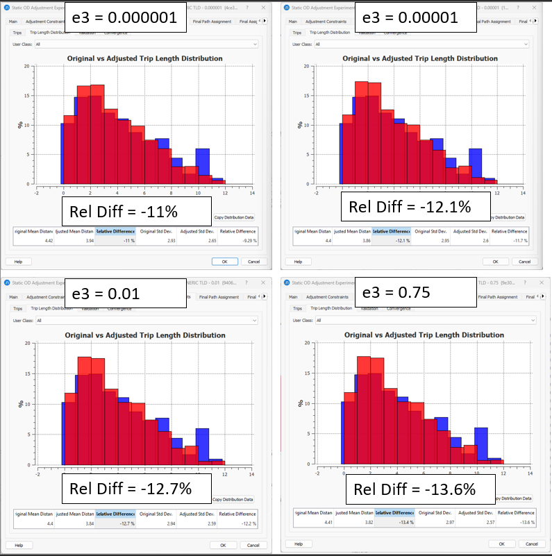
In a sample network, while keeping all the rest of the input parameters fixed, we tested the following 6 values of trip length distribution elasticities:

\(e_{1}\) = {0.000001, 0.00001, 0.01, 0.75}

To translate those elasticities into a weight (\(γ_{3}\)) used in the objective function, we apply the formula: \(γ_{3}= \frac{1}{e_{3}}-1\). 

\(γ_{1}\)= {999999, 99999, 99, 4}

See the comparison of the first iteration result (in blue) and the final result of the static OD adjustment (in red):

Again, these are just examples where the elasticity values tested were randomly chosen, so do not take those elasticity values as the default values for your project.

Demand Bounds

The Max Deviation Matrix can be used as a boundary to limit the variation of the new OD trips when calculated after each iteration. The demand bound value per OD cell works as a safety tool that aims to protect the adjustment process from moving far from the reference seed OD matrix.

Example:

For a single OD pair that goes from A to B:

• The seed OD Matrix has 100 trips
• The Detector measured at average 10 vehicles passing
• The Max Deviation Matrix is set to 50%, which means that the adjusted OD matrix can take values from 50 to 150 trips.

  After 1 iteration: 83 trips -> OK
  After 2 iteration: 64 trips -> OK 
  After 3 iteration: 35 trips -> adjusted to 50 trips
  After 4 iteration: 45 trips -> adjusted to 50 trips
  ...
  After N iteration: 22 trips -> adjusted to 50 trips
  

The Demand Bounds is a completely different concept from the Demand Elasticities.

Demand Bounds: I accept any change within the range defined. Which change? Up to the optimization algorithm using counts. I don’t care if it changes more or less.

Elasticity: I can accept any change. Which change? Up to the optimization algorithm using counts BUT penalizing if you deviate from the seed OD demand.

When demand bounds is set to Frozen, this is applied to limit the OD pairs. The demand bounds are applied at the last step of the adjustment in every iteration. So the value changes but then the constraints are applied. So in case of frozen ODs, their value will set back to the initial OD value (after every gradient descent step).