Distribution
The Distribution process transforms Generation/Attraction vectors, containing the total number of trips produced and attracted by each centroid, into OD matrices.
The algorithms used in undertaking the trip distribution calculations are explained in Demand Modeling and can be either a Gravity Model or a Destination Choice Model. See section Distribution Scenario and Experiment to see how to define the Distribution process.
If a prior matrix is known, an alternative option to update the matrix distribution to new totals is the Furness technique, available at the matrix editor as a matrix operation for factoring growth in origin and destination matrices.
Data and Functions
The data and model requirements for the Distribution Scenario and Experiment are:
- G/A Vectors.
- Skim Matrices.
- Distribution functions: Impedance and Deterrence functions for the Gravity model, Utility functions for the Destination Choice model.
- Distribution and Modal Split Areas.
- Distribution and Modal Split Data Sets.
Generation/Attraction Vectors
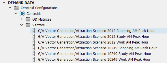
G/A vectors are the outputs from a Generation Attraction Experiment. They contain the number of trips generated in a centroid and the number of trips attracted to each centroid, by time period, trip purpose, transportation mode or all transportation modes.
Skim matrices
Skim matrices contain the costs between each OD pair. As the skim matrices are an output from an assignment experiment, they might not yet be available when starting the Four-Step model process. If no a priori estimation is available, they can be initially estimated with a basic All-or-Nothing assignment for each mode using a unit matrix as demand. These initial estimates will be updated with better estimates in subsequent iterations of the process.
Distribution Functions
The Distribution Impedance Functions are used to evaluate the impedance of a trip from one zone to another given the skim matrices of the available modes. The calculated impedance is passed into a Distribution Deterrence Function, which gives the values for the Gravity model.
Similarly, the Distribution Utility Functions are used to evaluate the utility of a trip in the Destination Choice model.
Distribution Functions are set in the Distribution Areas.
Distribution Macroscopic Areas 
Macroscopic areas are created to link sets of zones to demand related areas. The links are created in the Distribution and Modal Split tab of the Centroid editor. The process is:
- Create the Macroscopic Areas for Distribution and Modal Split and for Parking.
- For each Distribution and Modal Split Data Set, allocate Centroids to each area in the Distribution and Modal Split tab of the Centroid editor (this task can also be automatically done from the Distribution and Modal Split Data Set editor).
- Create the Distribution functions.
- In the Distribution and Modal Split Area editor, allocate the Distribution Functions to each Trip Purpose for each Distribution and Modal Split Data Set.
Distribution Area Editor
Distribution and Modal Split Areas set a classification for zones, i.e. Urban, Non Urban, etc. Areas are created in the Project folder Demand Data / Macroscopic Areas / Distribution and Modal Split Areas using the "New" option in the Demand Data context menu.
The Distribution Functions tabs are used to assign either Distribution Impedance functions or Distribution Utility functions to each trip purpose for the cases where there is a car available and no car available, or where no distinction is made. The functions are specified for each Distribution and Modal Split Data Set and Time Period.
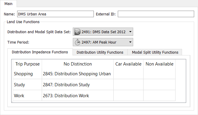
The Modal Split Functions tab is explained in the Modal Split Area editor section.
Each centroid is linked to a Distribution and Modal Split Area in the Centroid Editor: Distribution and Modal Split Tab.
Parking Area Editor
A Parking Area contains the cost and constraint parameters related to parking. Parking Areas are created in the Project Folder Demand Data / Macroscopic Areas / Parking Areas using the "New" option in the Demand Data context menu.
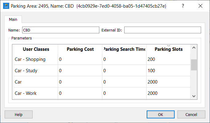
These values are specified per User Class (pair of vehicle type and trip purpose). The Parking Slots are only taken into account for Modal Split.
Distribution Data Sets
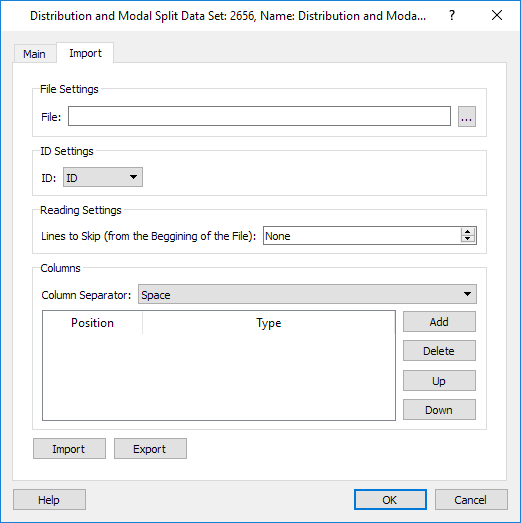
Distribution Data Sets allocate the Distribution data values to each centroid which can be read automatically from a text file in the Import tab. The Centroid ID setting specifies the type of ID that will be used to match centroids with the data with an external text file. It can be internal, external or name. The list of attributes is fixed:
- Distribution and Modal Split Area: The Distribution and Modal Split area this centroid is allocated to.
- Parking Area: The Parking area this centroid is allocated to.
- Use Parking Areas Costs and Search Times: A Boolean to opt to use the user defined parking parameters ( use 1 or true for "yes" or any other coding for "no").
- External: A Boolean that marks the centroid as external or not.
After setting the Centroid ID to be used, the number of files to skip, the separator format and the order of the columns in the file according to their content, press Import to import the data.

Distribution Data per Centroid
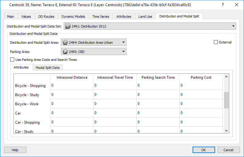
The Centroids Editor Distribution and Modal Split tab contains the data needed for the Distribution and for Modal Split calculations.
The type of Distribution Area and Parking Area for the zone are specified (they can be automatically imported from the Distribution Data Set editor). Also, for each user class, the values for Intrazonal Distance and Travel Time, and Parking Search Time and Parking Cost if they differ from the ones specified in the Parking Area editor. If they do differ, and the values specified here are the ones to be used, then the Use Parking Area Costs and Search Times checkbox must not be checked.
Distribution Scenario and Experiments
The Distribution Scenario and Experiment contain the data and parameters needed to run the trip distribution calculations.
The Distribution Experiment can use a Gravity model or a Destination Choice model. Which type of experiment is selected is determined as the experiment is created.
Distribution Scenario
The Distribution Scenario sets the input data for the distribution, which is the same for both experiments.
The Distribution Scenario contains only the basic scenario information.
To create a new Distribution Scenario, select New > Scenarios > Distribution Scenario in the Project Menu. If you are working on a subnetwork, the new scenario can be created from the subnetwork's context menu. The minimum requirement for a Distribution Scenario is a base transport network and a traffic demand.
The Scenario context menu has options to Activate, Delete, Rename, Duplicate or open the Scenario Properties editor.
When selecting Activate from a scenario, it is activated this scenario in the task tool bar area. Automatically it is activated the first experiment.
The scenario editor is divided into several tabs which describe what is to be simulated, the outputs to be collected, the variables used to modify the scenario, and some parameters to describe the scenario.
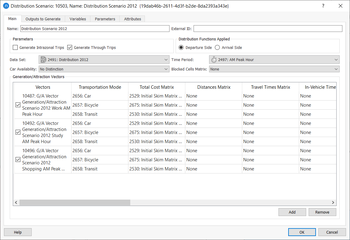
Intrazonal Trips and Through Trips will be generated, depending on the checkbox settings.
Each zone can be a different type of Distribution Area for which the corresponding Distribution functions have been specified. As each trip is related to two zones, an origin and a destination, it is necessary to specify whether to apply distribution functions depending on where the trip starts (usually for the morning peak) or where the trip ends (usually for the evening peak).
The Distribution Data Set, the Time Period and the Car Availability used to define the distribution must be selected.
In the Blocked Cells Matrix field, a matrix with contents Distribution: Blocked Cells can be selected. This auxiliary matrix will indicate which cells must be blocked during the process: a non-zero value in the auxiliary matrix will indicate a blocked cell. Blocking a cell implies that this cell will contain no trips in any of the output matrices. Note that this functionality is optional and complimentary to using a skim matrix with zero value (or empty) cells. A zero in a skim matrix is interpreted as 'impossible to reach' for the particular OD pair. But if the skim contains non-zero values and the cell is still to be blocked, a matrix containing the blockings can be selected here.
Select where to store the distribution results using the Outputs to Generate tab. If results are stored, the output matrices will be stored in a file with extension DIS.

If results are stored, they can be retrieved at any time after execution.
Distribution Experiment
To create a new Distribution Experiment, select New Experiment from the scenario context menu.
The Experiment context menu has options to Activate, Delete, Rename, Duplicate or open the Experiment Properties editor.When selecting Activate from a Experiment, it is activated this Experiment in the task tool bar area with the parent Scenario.
Two different models are available for Distribution calculation:
Gravity Model Experiment 
The algorithms for the Gravity model are described in the theory section on Distribution Models, specifically in the section on Gravity Models.
The main calculation behind the Distribution Model is to find multipliers \(M_{i}\) and \(N_{j}\) that meet the criteria:
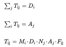
Where:
- \(i,j\) are the origin and destination indices.
- \(D\) and \(A\) are the trip volumes from origin \(i\) and destination \(j\).
- \(F\) is a deterrence function reflecting the cost of the trip \(i,j\).
The stopping criteria for the algorithm, that is, the Distribution Epsilon and the limit to the number of iterations, is set for the experiment together with the Deterrence Function.
The Network Attribute Overrides and pre- and post-run scripts are also specified here (optional).
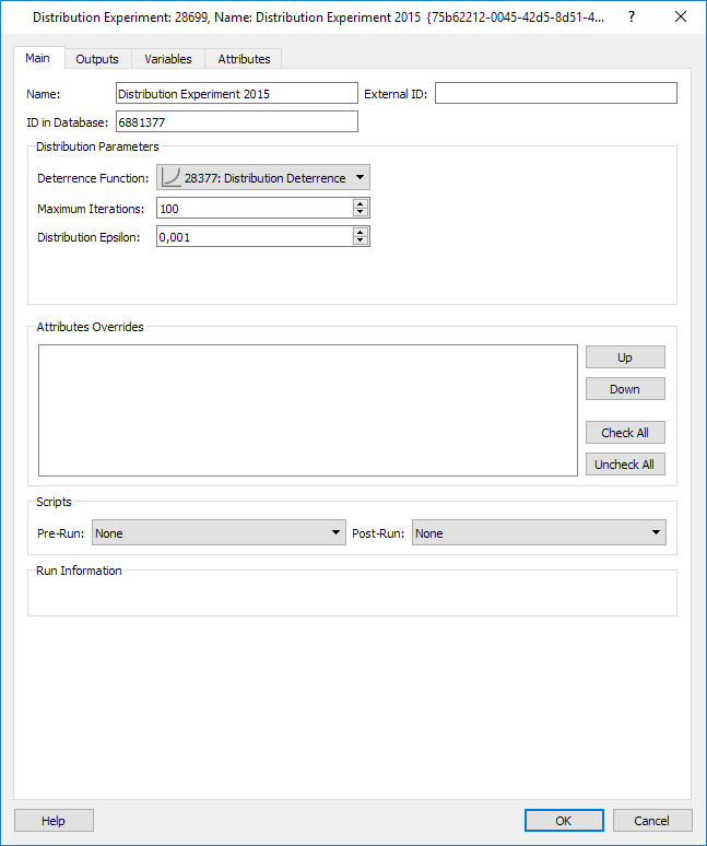
The Distribution algorithm is executed from the experiment context menu.
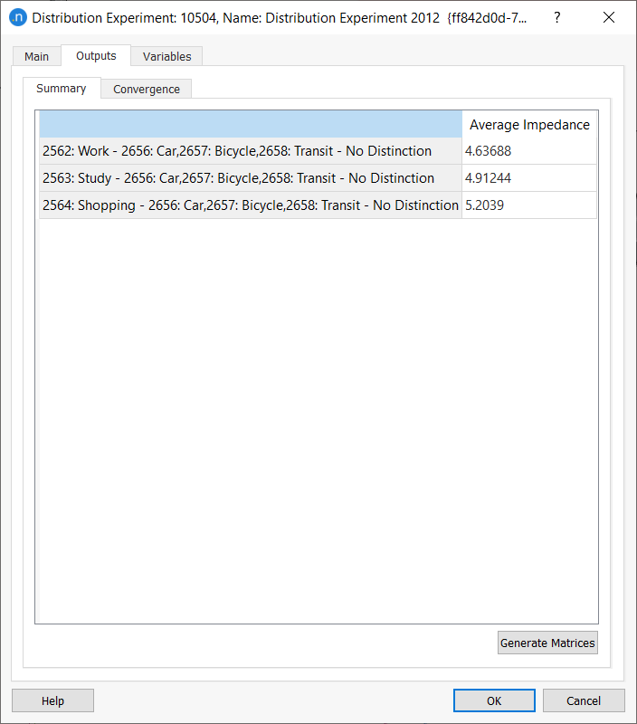
After the execution, the weighted mean impedance for each Individuals matrix will be available in the Outputs folder in the Experiment editor.
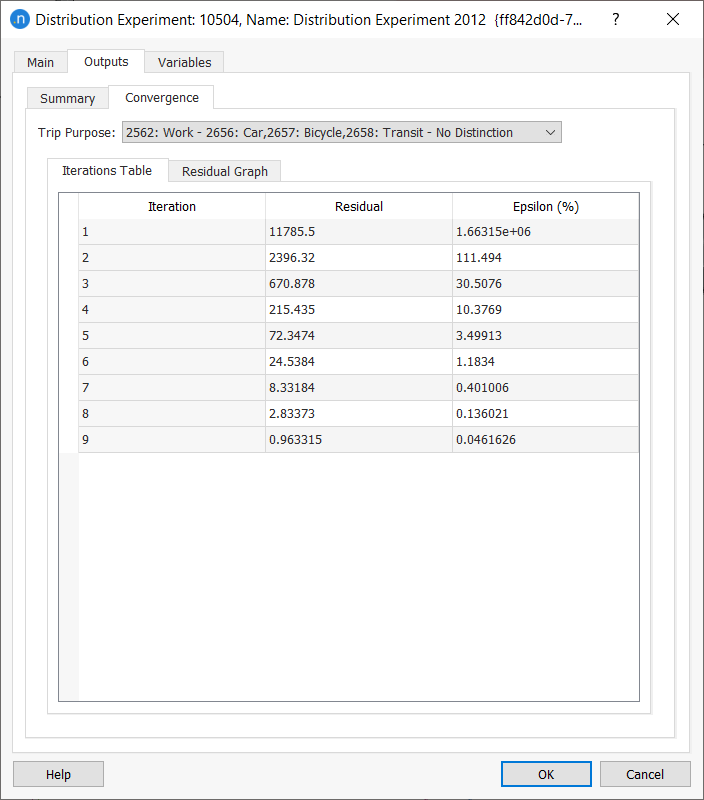
The Convergence tab displays the summary output to verify whether the process has converged to the desired provided Distribution Epsilon. The Distribution Epsilon is the stopping criteria and equivalent to the Furness process Epsilon. The Residual is the sum of the absolute differences between the values in the G/A vector and the totals in the OD matrix.
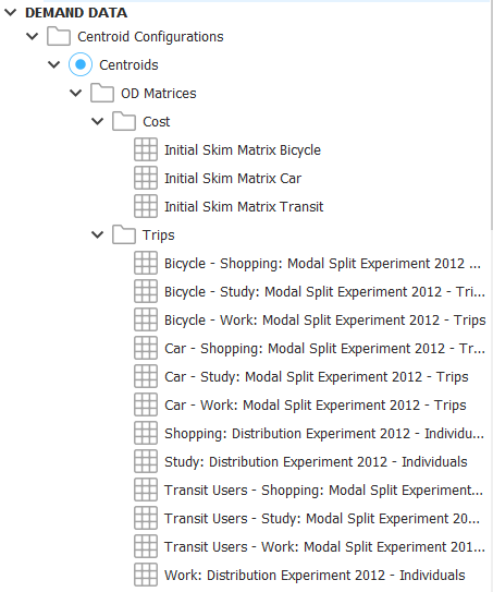
The Matrices for trips made by individual travelers can be created on demand from the experiment's Outputs / Summary tab, with the Generate Matrices option. The matrices will then be available under the list of OD Matrices in the corresponding centroid configuration.
Destination Choice Experiment
The algorithms for the Destination Choice model are described in the theory section on Distribution Models, specifically in the section on Destination Choice Models.
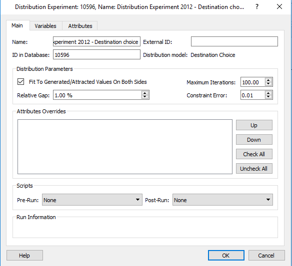
The Distribution experiment controls the iteration convergence criteria: maximum number of iterations, RGap and constraint factors.
The Network Attribute Overrides and pre- and post-run scripts are also specified here (optional).
The Distribution Utility functions are specified in the Macro Areas editor. These functions model the preferences or benefits of trips to all destinations available from each particular origin, in order to determine with a discrete choice multinomial logit the probability of traveling to a destination, and require data derived from external sources. This data can be stored in the Aimsun document as vectors or as matrices to give access to them in the function.