Static OD Departure Adjustment

The static OD departure adjustment is a procedure to create a profiled demand from a static demand. To obtain this profiled demand, the original static demand is distributed through smaller intervals over the time period. The objective is to reproduce the observed traffic counts specified in the Real Data Set per interval, staying as close as possible to the original number of OD pair trips for the whole period.

Thus, it is important to start the process with a calibrated demand that fits the detection data over the scope of the model. The static OD departure adjustment does not calculate any new assignment, it takes previously calculated fixed paths from a Path Assignment produced earlier and link (section + turn) travel times, which are used to calculate the assigned number of vehicles for each time period. The method employed by the static OD departure adjustment scenario is described in Static OD Departure Adjustment Algorithms.

To execute a static OD departure adjustment, create a Static OD Departure Adjustment Scenario object and add an Experiment to it. The scenario will contain all the input data; an experiment created from this scenario will contain the algorithm parameters.

The result of the OD departure adjustment will be a set of matrices that form a profiled Traffic Demand.

Static OD Departure Adjustment Scenario

The Static OD Departure Adjustment Scenario editor contains the input data for the departure adjustment execution.

To create a new Static OD Departure Adjustment Scenario, select New > Scenarios > Static OD Departure Adjustment Scenario in the Project Menu. If you are working on a subnetwork, the new scenario can be created from the subnetwork's context menu. The minimum requirement for a Static OD Departure Adjustment Scenario is a base transport network and a traffic demand.

The Scenario context menu has options to Activate, Delete, Rename, Duplicate or open the Scenario Properties editor.

When selecting Activate from a scenario, it is activated this scenario in the task tool bar area. Automatically it is activated the first experiment.

The scenario editor is divided into several tabs which describe what is to be simulated, the outputs to be collected, the variables used to modify the scenario, and some parameters to describe the scenario.

Main tab

The main tab defines the scenario in particular, the Traffic Demand and the Warm-up duration, the Path Assignment Plan, and the Real Data Set. You can also activate the Geometry Configurations for this scenario.

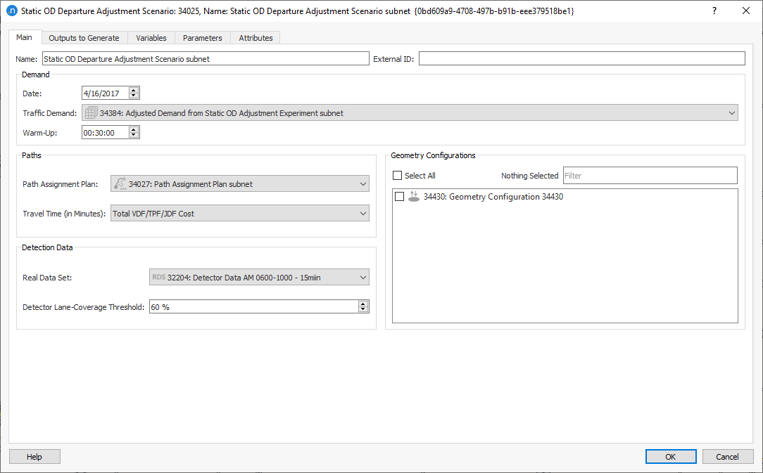
Demand

The initial traffic demand can be a single matrix covering the whole period; there is no requirement to profile it before running the OD departure adjustment experiment. This is included as the first step in the process to split the matrix into multiple matrices using the time intervals in the real data set. So if the data contains counts at 10-minute intervals, a 1-hour prior OD matrix will be split into 6 matrices which will be initialized with 1/6 of the overall demand.

Because the departure adjustment takes into account the travel time from origin to detectors, the results for the first time intervals might be unrealistic if the network is not correctly loaded with vehicles at the start of the assessed period. Therefore, a warm-up time is recommended and the traffic demand will then be automatically extended to operate before its initial time.

If there is detection data for the warm-up period, the demand for the warm-up will be allocated a matrix in proportion to the total vehicle count in the warm-up period and the modeled period. If no detection is available for the warm-up, it will receive a flat demand equal to the initial estimated profiled demand for the first interval.

Paths

The paths information is defined by specifying a Path Assignment Plan obtained from a static assignment or a static OD adjustment. The travel time is calculated with the assumption that the generalized costs of the path assignment represent solely the travel time and that it is provided in minutes.

If this is not the case, e.g. when the generalized cost includes a toll or a distance component or the cost units are not in minutes, a Function Component must be defined in the static cost functions to provide the travel time in minutes. This Component must then be selected in the Travel Time (in minutes) field.

Detection Data

The detection data is defined by specifying the Real Data Set that contains the counts from Detectors or Detector Stations in the network. The Detector Lane Coverage Threshold determines the percentage of lanes a detector and/or detector station must cover in order to be included in the adjustment process.

Static OD Departure Adjustment Experiment

Create a new Static OD Departure Adjustment Experiment by right-clicking on the Static OD Departure Adjustment Scenario.

The Experiment context menu has options to Activate, Delete, Rename, Duplicate or open the Experiment Properties editor.When selecting Activate from a Experiment, it is activated this Experiment in the task tool bar area with the parent Scenario.

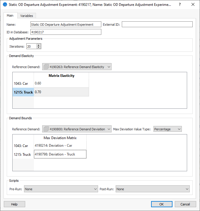
On the Main tab, specify the following parameters:

• Number of Iterations to be performed.
• Demand Elasticity per user class: A value between 0 and 1 to indicate the elasticity of the adjusted demand with respect to the Reference Demand. A zero value (not allowed by the UI) means that no variation is allowed and a value of 1 means that variation is not penalized at all. The default value is 0.5. This means that equal weighting is applied to the dual goals of maintaining the prior matrix value and matching the detector values.
• Demand Bounds: Maximum Deviation Matrix, per user class. Maximum Deviation Value Type: Select Percentage, Factor, or Absolute, and specify a Max Deviation Matrix (with Contents: Max Deviation) per user class (Car, Truck, etc.) to limit the changes in the traffic demand with respect to the Reference Demand. Leave as None if no demand bounds are specified. Refer to Adjustment Maximum Deviation Section for more information.
• Scripts: Select Pre-Run and Post-Run scripts, if applicable, to run before and after the experiment.

The experiment/process can be run from the context menu of the Static OD Departure Adjustment Experiment.

Static OD Departure Adjustment Outputs

Trips

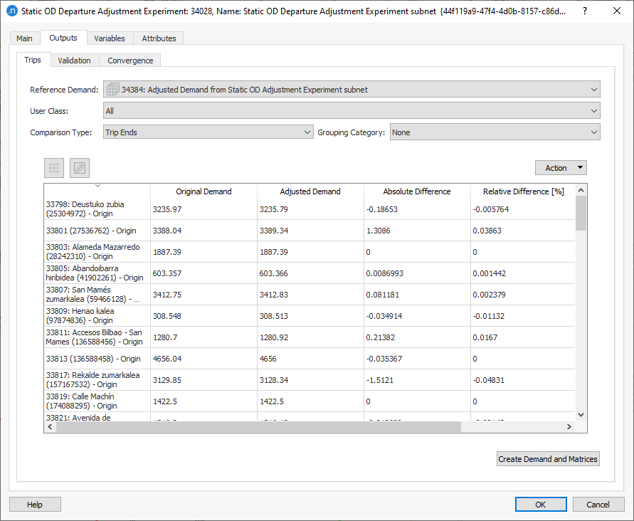
The result of the Departure Adjustment is a set of profiled matrices, with the same interval as the data in the Real Data Set. Create the new Traffic Demand to include these OD matrices by clicking the Create Demand and Matrices button.

The adjusted matrices from the experiment are displayed on the Trips subtab. They are presented by User Class (which can be changed to other User Class or to All) and include Original Demand, Adjusted Demand, Absolute Difference, and the Relative Difference [%]. Click the demand column headings to sort the rows by quantity of demand and difference.

A drop-down that allows choosing whether the comparison should be input traffic demand or other Reference demand (if other traffic demands are selected in the Main tab, under Demand Elasticity and Demand Bounds) vs. adjusted.

A drop-down menu allows the user to select Cell-by-cell or Trip Ends to compare the number of generated and attracted trips per centroid or filter per Grouping Category. The total number of rows is equal to the number of rows + number of columns of the centroids in the Traffic Demand object.

To plot Trips outputs as a regression line, comparing adjusted and original demand, click the graph icon .

To create the new travel demand and its matrices, click Create Demand and Matrices. The new demand and matrices will be stored in the Project folder.

In the graph, the total adjusted demand (by user class if selected) is compared with the original demand in tabular form or as a regression plot as shown here.

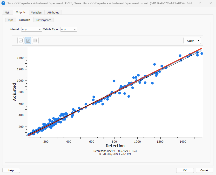
To copy the data or save a screenshot of the data, click Action and select Copy Table Data or Copy Graph (Snapshot). You can now paste the saved data or graphic into other applications for analysis or display.

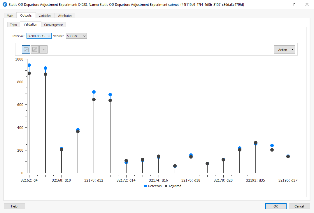
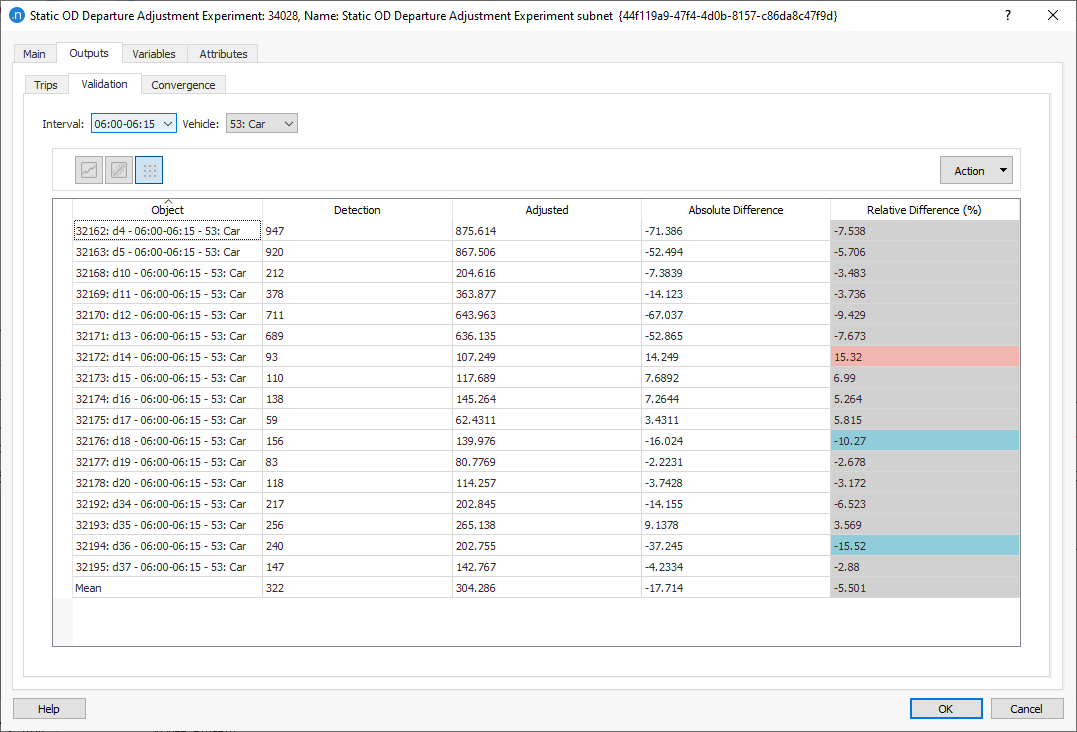
Validation

The Validation tab is used to compare the results (only the last iteration) with the Real Data Set. Results for all intervals or for a selected interval and for all vehicles types or for a selected one are shown as a regression plot, as a table, or, as shown here, as a stick plot. Results can be filtered by interval and/or vehicle type selecting the desired one in the corresponding combo box located at the top of the dialog.

Convergence

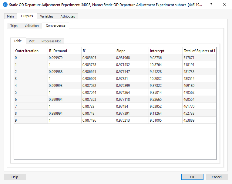
The Convergence subtab displays the progress toward the convergence of the R² value and the relative gap of the assignment at each iteration.

• Outer Iterations. The number of iterations specified in the experiment for Maximum Number of Iterations.

• R² Demand. The measure of the closeness of the fit of the adjusted demand and the seed demand.

• R². The measure of the closeness of the fit of modeled flows to observed flows.

• Slope and Intercept. The two values defining the regression line.

• Total of Squares of Errors. The sum of the squares of observed–modeled flows.

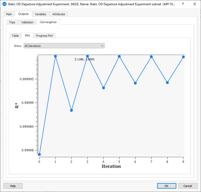
The Plot tab shows the progression of the R² value per iteration. If it has converged on a value close to 1.0 then the adjustment can be considered complete. If it is still rising toward 1.0 then more iterations might be required. If it is stabilizing at a value much lower than 1.0 then the input matrix, and its constraints, are preventing the adjustment procedure from achieving a satisfactory result.

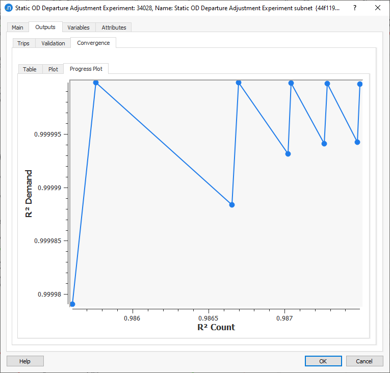
The Progress Plot tab shows the progression of the R² Demand value and the R² value per iteration. This plot shows the effect of each adjustment step both in terms of distorting the seed matrix and in terms of improving the validation.

The screenshots below show the Table, the Plot and the Progress Plot subtabs.