Dynamic OD Adjustment

A dynamic OD adjustment is a procedure to refine a set of prior matrices (profiled demand) with traffic counts from a real data set. The dynamic OD adjustment uses a gradient descent method to iteratively adjust the traffic demand in each time interval, using the outputs of a dynamic simulation.

Each time interval is adjusted in turn using a rolling horizon where earlier intervals are adjusted first to ensure the prior conditions are properly set for the interval being adjusted. The dynamic OD adjustment methodology and algorithms are documented in the Dynamic OD Adjustment Algorithms section. The result of the dynamic OD adjustment is a new set of integer matrices that form a profiled traffic demand.

For a wider theoretical explanation about matrix adjustment, see Estimation of OD Demand Flows Using Traffic Counts: Matrix Adjustment.

The dynamic OD adjustment is based on a dynamic simulation which can be implemented as a microsimulation, a mesoscopic simulation, or as a hybrid simulation. This is because paths chosen by vehicles are independent of the means by which they are moved through the network.

Like the static OD adjustment, the dynamic OD adjustment is iterative and has two levels of calculations. First, the inner layer runs a dynamic assignment to generate paths and link flows, assigning the set of OD matrices in the current iteration to the network. The dynamic assignment uses the method and parameters specified in the experiment's Dynamic Traffic Assignment tab, which are the same as in a standard simulation experiment.

Second, a gradient descent step adjusts the OD matrix using the paths and flows obtained in the static assignment.

Data and Preconditions

Prior Matrices

The traffic demand specified in the scenario must split the prior matrices by user class and by time slice. The same structure of OD matrices will be used in the adjusted matrices.

If the original demand consists of a flat matrix per vehicle type, for a single time period, it should be split into smaller time slices using OD matrix editing tools. Alternatively, a static OD departure adjustment should be applied first and a new Traffic Demand object created with the sliced matrices.

Real Data Set

The real data set used in the dynamic OD adjustment will specify the observed traffic counts. These can be traffic counts for detectors, detector stations, road sections, turns contained in nodes or subpaths from the same period as the demand period to be adjusted. The demand slice duration should be a multiple of the interval times of the real data set traffic counts. Otherwise, the dynamic OD adjustment will not be executed.

If detector or detector station counts are used, these will be converted to section counts using a linear extrapolation if the section and the detector have different numbers of lanes. For example, a detector covering two of the three lanes of its section, having an observed count of 500 vehicles, will be converted into a section count of 3/2 x 500 = 750 vehicles. If the counts are expressed by user class, these must be the same classes as specified in the prior matrices.

If subpaths counts are used, the RDS count will be taken into account consistently as the subpath statistics, that is, for the amount of vehicles that follow all sections and turns of the subpath during its trip.

The real data set can include a Reliability value per each detection value. This value is taken into account in the adjustment process as a weight for the difference between observed and assigned counts (that is, the bigger the Reliability, the more effort the adjustment will make to match that particular pair of values). If no reliabilities are set, they are assumed to be 1.0 by default.

An extra column named Congested can be included in the real data set. This column specifies, for each count, whether this count is observed under congested conditions (1) or uncongested conditions (0). If this data is not specified, the count is considered to be observed under uncongested conditions.

Road Network

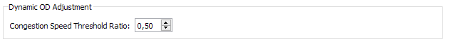
In the Dynamic Models tab of each road section, there is a parameter named Congestion Speed Threshold Ratio. This parameter indicates below which factor of speed a section is considered to be congested in the simulation. A default value of 0.5 will be used (e.g. on a section with a default congestion speed threshold ratio of 0.5, and a speed limit of 80 km/h, the section is considered to be congested for a particular statistical interval if the average simulated speed of that interval drops below 40 km/h).

Effects of Congestion on the Adjustment Calculation

One of the aims of an adjustment is to be able to replicate congestion. Congestion can be detected in the observed data or in the simulation, producing the following possible situations and actions.

• If there is congestion in the observed data but not in the simulation: the current simulated value is targeted to be increased by the Demand Increase to Reach Congestion percentage.
• If there is no congestion in the observed data but congestion in the simulation: the current simulated value is targeted to be decreased by the Demand Increase to Reach Congestion percentage.
• If there is congestion in both observed and simulation data: an increase in demand will lead to a decrease in flow and vice versa. The current simulated value is targeted to be increased or decreased, depending on the difference between simulated and observed congestion, by the Demand Increase to Reach Congestion percentage.

Dynamic OD Adjustment Scenario

A dynamic OD adjustment scenario needs a dynamic OD adjustment experiment. The scenario contains the input data for the adjustment: the prior matrices in a traffic demand, the control plan, the transit plan, and any geometry configurations. The parameters for the scenario are set in the same manner as for any dynamic scenario, with the proviso that a real data set must be specified, with a format that includes the time, location, count, and any additional congestion data required for the adjustment experiment.

Dynamic OD Adjustment Experiment

The Dynamic OD Adjustment Experiment dialog contains all the algorithm parameters. To create a dynamic OD adjustment experiment, right-click on the scenario and select New Dynamic OD Adjustment Experiment. As with a Dynamic Assignment Experiment, you are required to choose the network-loading method (mesoscopic simulation, microscopic, hybrid meso-micro, or hybrid macro-meso) and the path assignment method (stochastic route choice or dynamic user equilibrium).

Next, configure the dynamic OD adjustment experiment for simulation behavior, reaction times, traffic arrivals, assignment parameters, traffic management policies, and other variables and attributes. This process is the same as for any other Dynamic Experiment but the dynamic OD adjustment experiment has an extra tab named Adjustment Parameters. This enables you to control the adjustment process.

Adjustment Parameters Tab

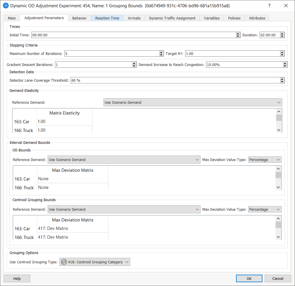
The Initial Time is the interval at which the process will start adjusting the demand. Matrices earlier than this time will not be adjusted and will remain the same as the originals.

The Duration marks the interval after which the process will stop adjusting the demand. Matrices later than the set time will not be adjusted and will remain the same as the originals.

For each of the time intervals, the Maximum Number of Iterations (or a lower number if the Target R² is reached) is completed before moving onto the next interval. In each iteration, the process will run a dynamic assignment and use the paths and path percentages obtained from it.

The number of Gradient Descent Iterations indicates, for each iteration of the adjustment, how many iterations of the gradient descent method will be run without changing the path-choice results: that is, without running a new assignment. The default number of these is 1, which implies that a dynamic traffic assignment will be run at each iteration of the adjustment.

Assuming that the path percentages do not change significantly at each iteration, you can reduce computing time by increasing the Gradient Descent Iterations and decreasing the Maximum Number of Iterations.

The Demand Increase to Reach Congestion field specifies the percentage increase to be targeted in the different cases of congestion already mentioned.

The Detector Lane-Coverage Threshold specifies the percentage of lanes that a detector and/or a detector station should cover in order for its data to be included in the adjustment process.

In the Demand Elasticity group box, the Matrix Elasticity indicates the elasticity of the adjusted matrix, for each user class, with respect to the Reference Demand selected above it (which is, by default, the Scenario Demand). Elasticity can have a value from 0.01–1.0. Trips comparison is one of the adjustment outputs and the significance of this comparison is controlled through the Matrix Elasticity parameter.

A Matrix Elasticity value close to 0 means that the values in the adjusted matrix will be almost unchanged from the previous matrix for that user class. An elasticity value of 1.0 means that no penalization has been applied to the amount by which the value can be adjusted to match the observed counts.

The Reference Demand parameter allows the user to select a different reference demand from the one being adjusted. This is important to consider when doing a multi-step process as part of the matrix adjustment. The Reference Demand must have the same user classes duration as the scenario's traffic demand. If the reference demand has a different slicing of demand, then the sum of trips across all slices for each OD pair and user class are used from the reference demand for elasticities.

In the Interval Demand Bounds group box, the constraints for the adjustment can be specified. In the OD bounds box, the user can specify a Maximum Deviation Matrix specify, for each user class, the deviation from the Reference Demand that is permitted. It can be specified as a Percentage, an Absolute Value, or Factor in the drop-down list labelled Max Deviation Value Type. See Adjustment Maximum Deviation Section for more details.

If the reference demand has the same slicing of demand as the scenario’s traffic demand, then the maximum deviations will be used for each user class and interval separately. If the reference demand has a different time-slicing to the scenario demand, then the deviation will be considered iteratively for each user class and interval. If after adjusting an interval, the change to an OD pair is not constrained by the deviation, the remaining deviation will be distributed proportionately again among the intervals waiting to be adjusted. This iterative procedure ensures that the sum of all upper (and lower) bounds is exactly equal to the total upper (and lower) bounds for each OD pair.

It is also possible to specify constraints and elasticities by sector using a grouping category for centroids. This reduces makes the adjustment less sensitive to route choice and reduces the probability of indiscriminate infilling. The user must specify a grouping category in the Grouping Options box using the Use Centroid Group Type drop down list. By specifying a centroid grouping category, the centroid groupings are also considered in the elasticities.

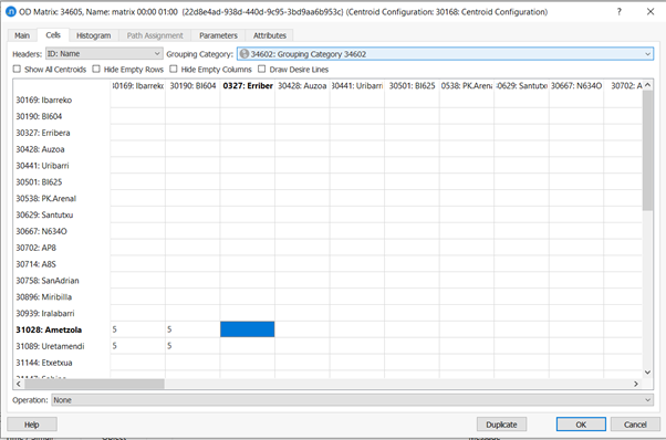
To specify a sector-to-sector maximum deviation, the user must create a maximum deviation matrix with a grouping category.

Then, in the Interval Demand Bounds > Centroid Grouping Bounds, select the maximum deviation sector to sector matrix.

Variables Tab

The Variables tab enables you to define values that are not defined in the dynamic OD adjustment scenario dialog, or to define different values than those set in the scenario. Variables specified in the experiment take priority over the same variables in the scenario.

To start every gradient descent with the prior matrix instead of the current matrix, add the variable $FIX_PRIOR_MATRIX to the experiment and set its value to TRUE. This approach should only be used when complying with UK Department for Transport (DfT) guidelines.

Dynamic OD Adjustment Replication

To execute the dynamic OD adjustment, first right-click on the adjustment experiment and select New Replication. The parameters to set for this replication are the same as those for a dynamic replication (or, for a result, they are the same as those for a dynamic result).

To run the replication, right-click it and select Run Dynamic OD Adjustment. When the replication finishes, the Dynamic OD Adjustment dialog is displayed. The tabs and subtabs of the dialog that contain outputs are described below.

Outputs Summary

The Outputs Summary tab is the same as for a dynamic assignment replication.

Validation

The Validation tab is the same as for a dynamic assignment replication.

Time Series

The Time Series tab is the same as for a dynamic assignment replication.

Path Assignment

The Path Assignment tab is the same as for a dynamic assignment replication and is described in Path Analysis Tool.

Adjustment Output

The Adjustment Output tab contains four subtabs: Trips, Vehicles, Convergence, and Validation.

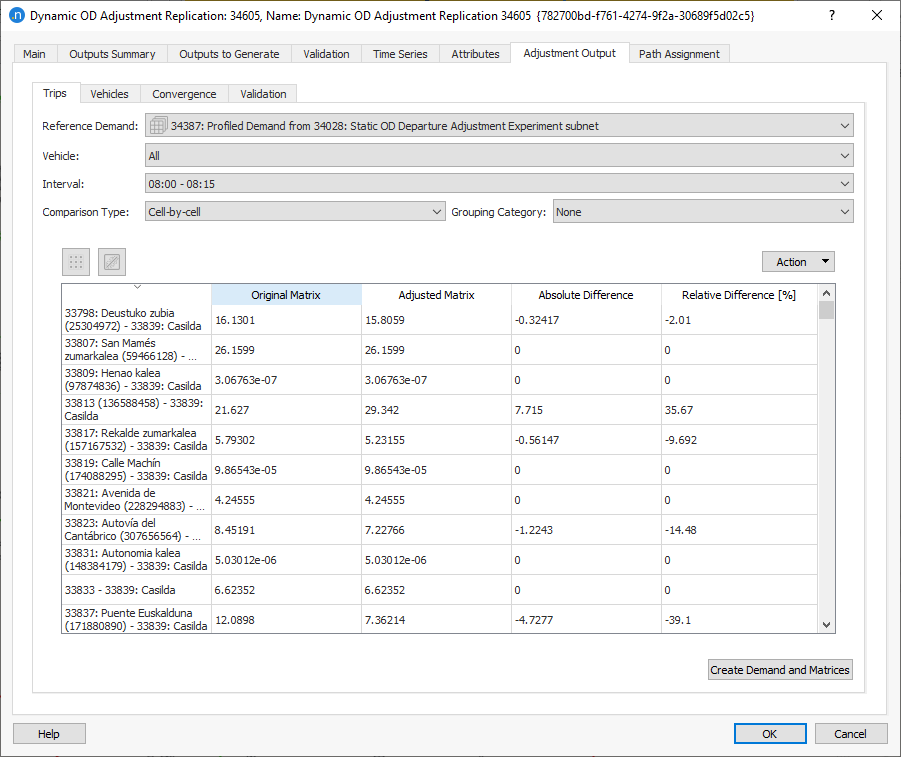
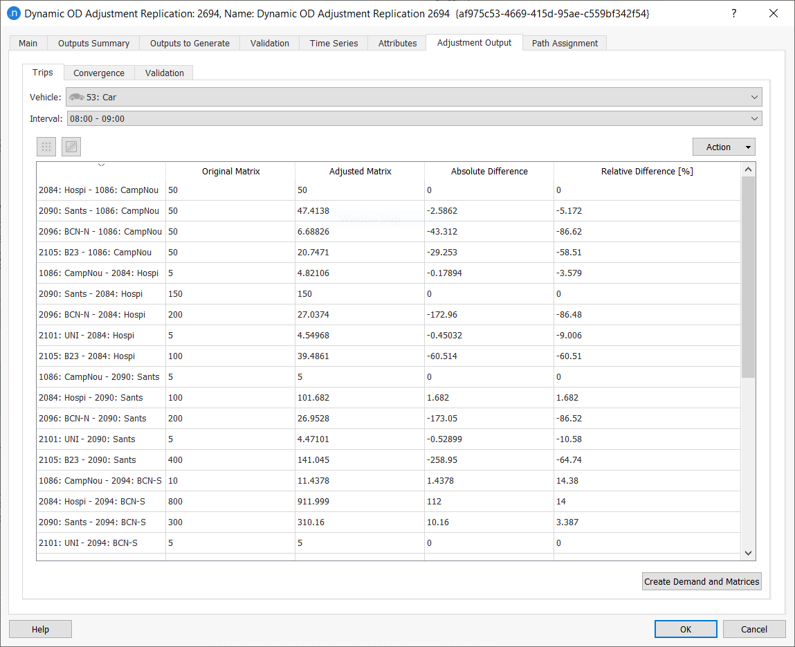
Trips Subtab

The adjusted matrices from the experiment are displayed on the Trips subtab. They are presented by User Class (which can be changed to other User Class or to All) and include Original Demand, Adjusted Demand, Absolute Difference, and the Relative Difference [%]. Click the demand column headings to sort the rows by quantity of demand and difference.

A drop-down that allows choosing whether the comparison should be input traffic demand or other Reference demand (if other traffic demands are selected in the Experiment under the Adjustment Parameters tab, under Demand Elasticity and Interval Demand Bounds) vs. adjusted. If the reference has not the same slicing as the input, the comparison with the reference is done aggregating all time periods.

A drop-down menu allows the user to select Cell-by-cell or Trip Ends to compare the number of generated and attracted trips per centroid or filter per Grouping Category. The total number of rows is equal to the number of rows + number of columns of the centroids in the Traffic Demand object.

To plot Trips outputs as a regression line, comparing adjusted and original demand, click the graph icon .

To create the new travel demand and its matrices, click Create Demand and Matrices. The new demand and matrices will be stored in the Project folder.

The Trips subtab shows the adjusted demand compared with the reference demand for each Vehicle and time Interval.

To copy the data or save a screenshot of the data, click Action and select Copy Table Data or Copy Graph (Snapshot). You can now paste the saved data or graphic into other applications for analysis or display.

Vehicles Subtab

The Vehicles subtab displays original and adjusted integer demand about vehicles in a table and/or time series. It can be filtered by vehicle type and time interval. This subtab is similar to the Trips subtab but uses actual generated vehicles.

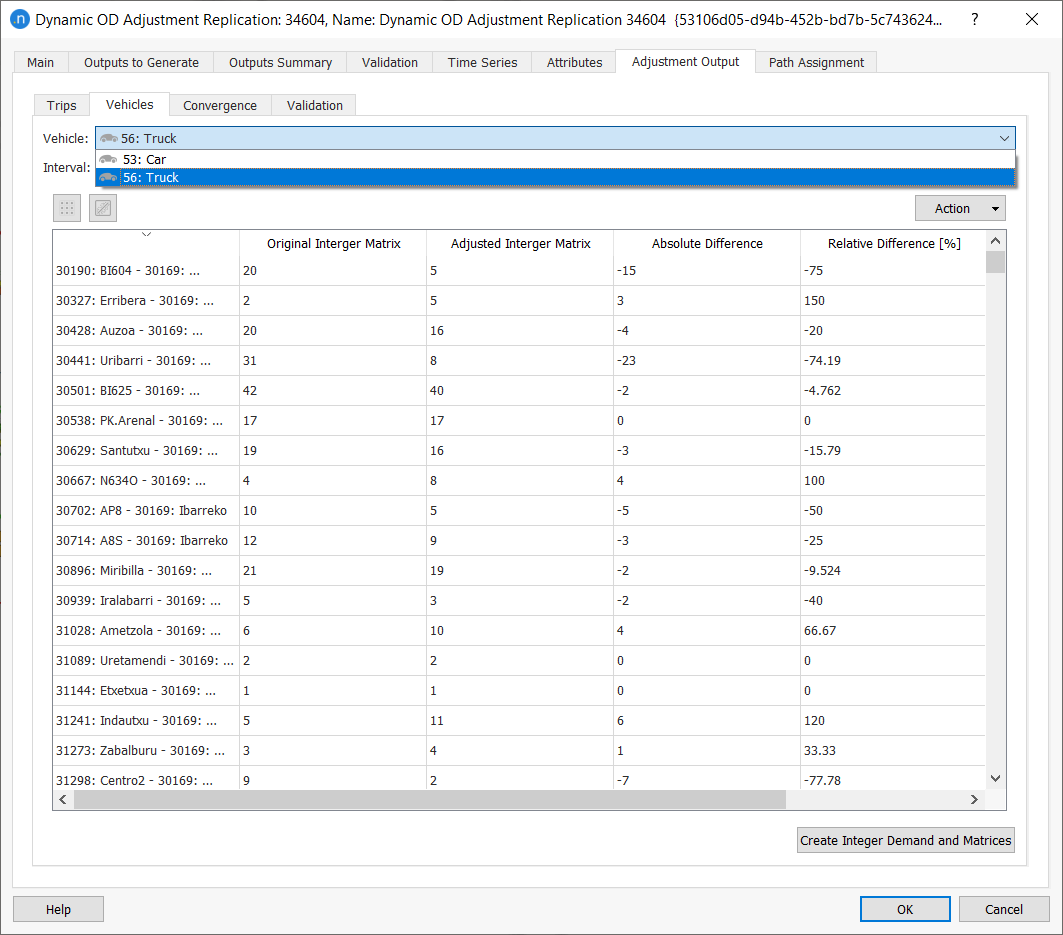
The data can be viewed in table form or as a time series by clicking the table and graph icons.

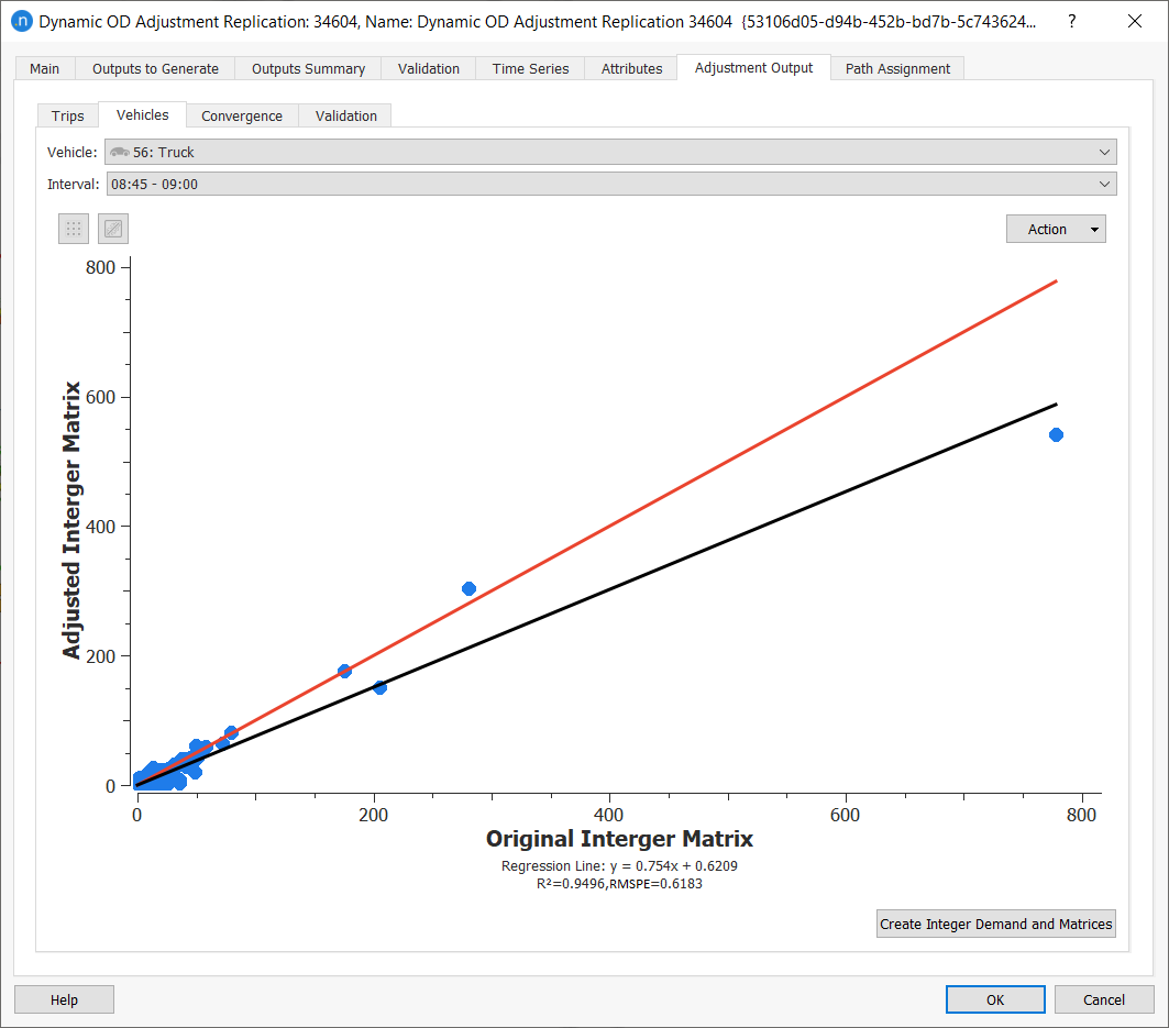
Click Create Integer Demand and Matrices to output integer OD matrices.

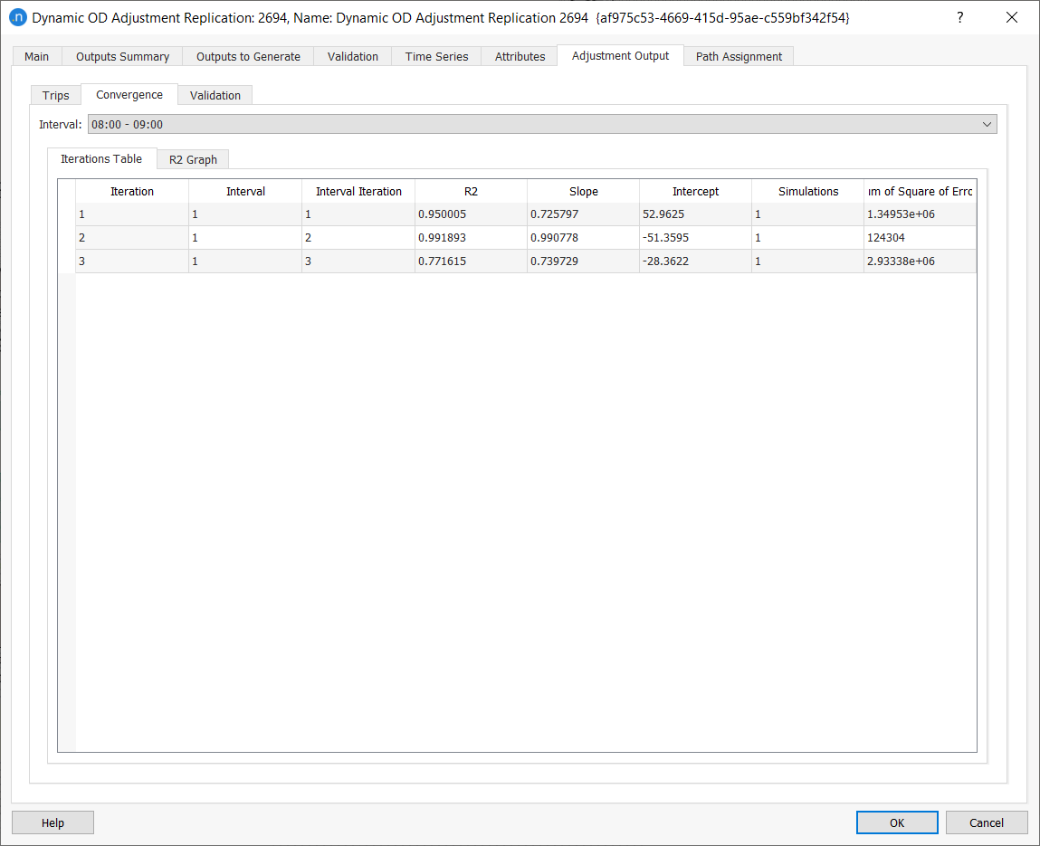
Convergence Subtab

The Convergence subtab displays information about the evolution of the R²v value for each iteration of each interval.

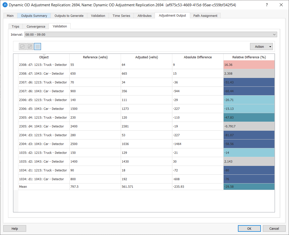
Validation Subtab

The validation tab displays the comparison between the measurements used by the adjustment process and the final simulated values (using the adjusted demand) associated with each of them. To view the data for different time intervals, click Interval to select from the drop-down list.

The data is presented as a table but to view it as a line graph, click .

To view it as a regression plot, click .

To copy the data or save a screenshot of the data, click Action and select Copy Table Data or Copy Graph (Snapshot). You can now paste the saved data or graphic into other applications for analysis or display.