Modeling with Macroscopic Tools
Note about licenses: These exercises require a license for Aimsun Next Advanced, Expert, or Pro TDM Editions.
- Exercise 1. Assigning an OD Matrix to a Network
- Exercise 2. Adjusting an OD Matrix
- Exercise 3. Calculating Traversal Matrices
- Exercise 4. Balancing Matrices
Introduction.
In these exercises, we will become familiar with some of Aimsun Next's macroscopic modeling tools. We will begin by assigning an OD matrix to a network to see how the flow distribution is assigned and how results are obtained. Next we will adjust the OD matrix by using real data from detectors. Then we will define a subnetwork for which we will obtain a traversal OD matrix. Finally, we will study an example of how to balance an OD matrix using the Furness method.
The backup copies of the files related to this exercise are in [Aimsun_Next_Installation_Folder]/docs/tutorials/6_Macroscopic_Modelling.
Exercise 1. Assigning an OD Matrix to a Network
1.1 Setting up the scenario and experiment
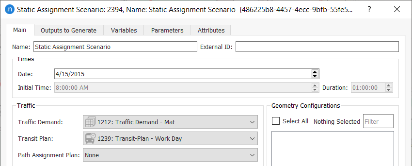
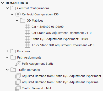
For this exercise, the traffic demand Traffic Demand – Mat is already defined and contains two OD matrices, one for cars and another for trucks. We will add this demand to the scenario.
To set up the scenario and experiment:
-
Open Initial_Macroscopic_Modelling.ang.
-
In the Project folder, right-click Scenarios > New > Static Assignment Scenario.
-
Open the new scenario.
-
For Traffic Demand, select Traffic Demand – Mat.
-
For Transit Plan, select Transit-Plan Work Day. This means that the additional fixed volume that Transit vehicles represent will be included in the assignment calculations.
-
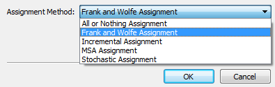
Right-click the scenario and select New Experiment, select the Frank and Wolfe Assignment type, and click OK.
-
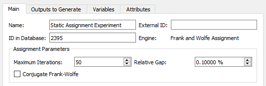
Open the experiment and for Maximum Iteration, enter 50, and for Relative Gap, enter 0.1000.
-
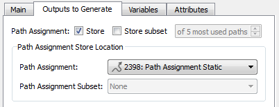
To create a path assignment object to save the paths from the static assignment, right-click Demand Data > New > Path Assignment.
We might want to use the saved paths later in other dynamic scenarios (see for example the exercises in the Integrating tutorial).
-
Rename the new object Path Assignment Static.
-
To link the path assignment object to the static assignment experiment, open the experiment, tick Path Assignment and, from the Path Assignment drop-down list, select Path Assignment Static.
-
To run the simulation, right-click the experiment and select Run Static Traffic Assignment.
1.2 Viewing the outputs
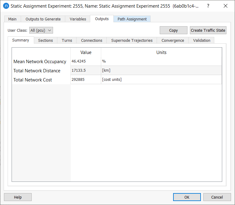
When the simulation finishes, the results dialog is displayed.
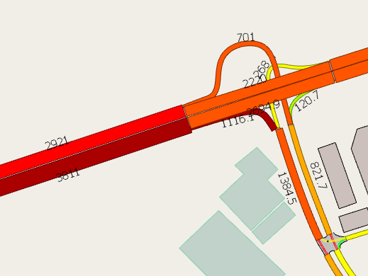
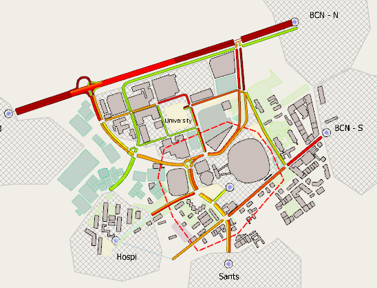
The first results are assigned vehicle volumes and they are displayed in the 2D view, as shown below.
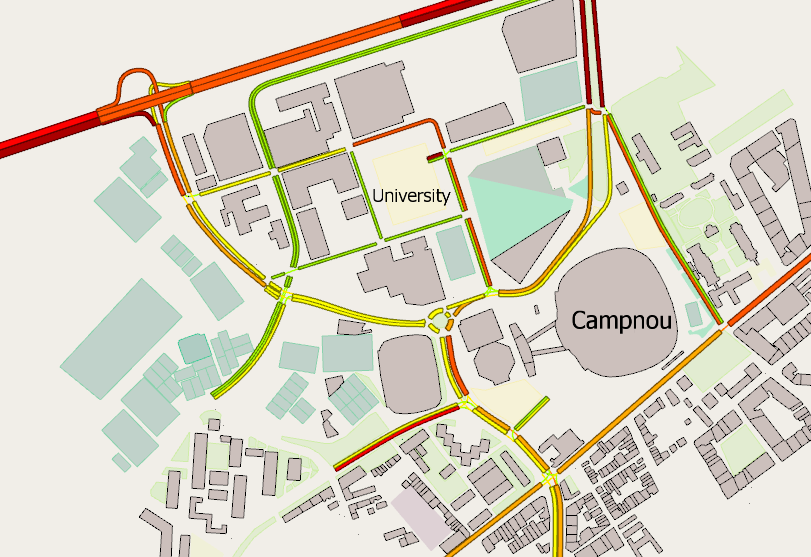
The values displayed on each section for the vehicle type All are the assigned section volumes in PCUs (passenger car units), where different sizes of vehicles are assigned different equivalent car weightings.
For example, 1596 PCUs are assigned to exit the network at the Sants centroid. In the matrices, there are 1300 cars and 140 trucks:
1300 * 1 PCU + 140 * 1.9 PCU = 1566 PCU
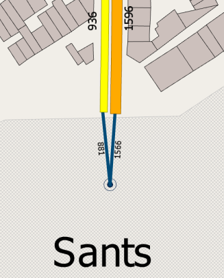
The assigned volume is 1596 and not 1566 because there are 12 buses in this section, which are weighted at 2.5 PCUs each. This accounts for the extra 30 PCUs.
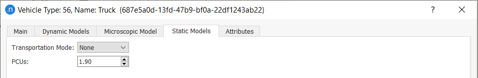
The PCU weighting of each vehicle type is defined, and can be changed, in the Vehicle Type dialog on the Static Models tab.
The width of the colored bars in the 2D view also indicates the volume assigned to sections. The color scaling indicates the ratio of volume:capacity for each section. The more congested sections are those with darker colors.
To view more results:
-
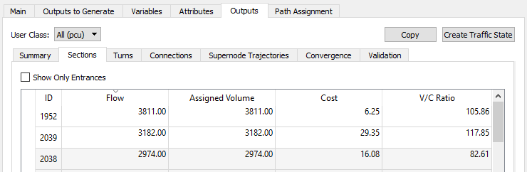
To view the volume and travel times per section and per vehicle type, click the Outputs tab and then the Sections subtab.
-
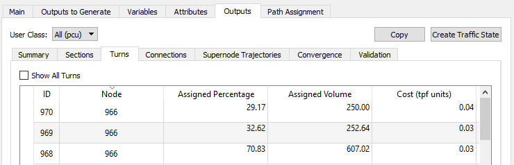
Click the Turns subtab to view section-to-section turn percentages and volumes.
-
Change the User Class from All to Cars or Trucks to filter the results.
-
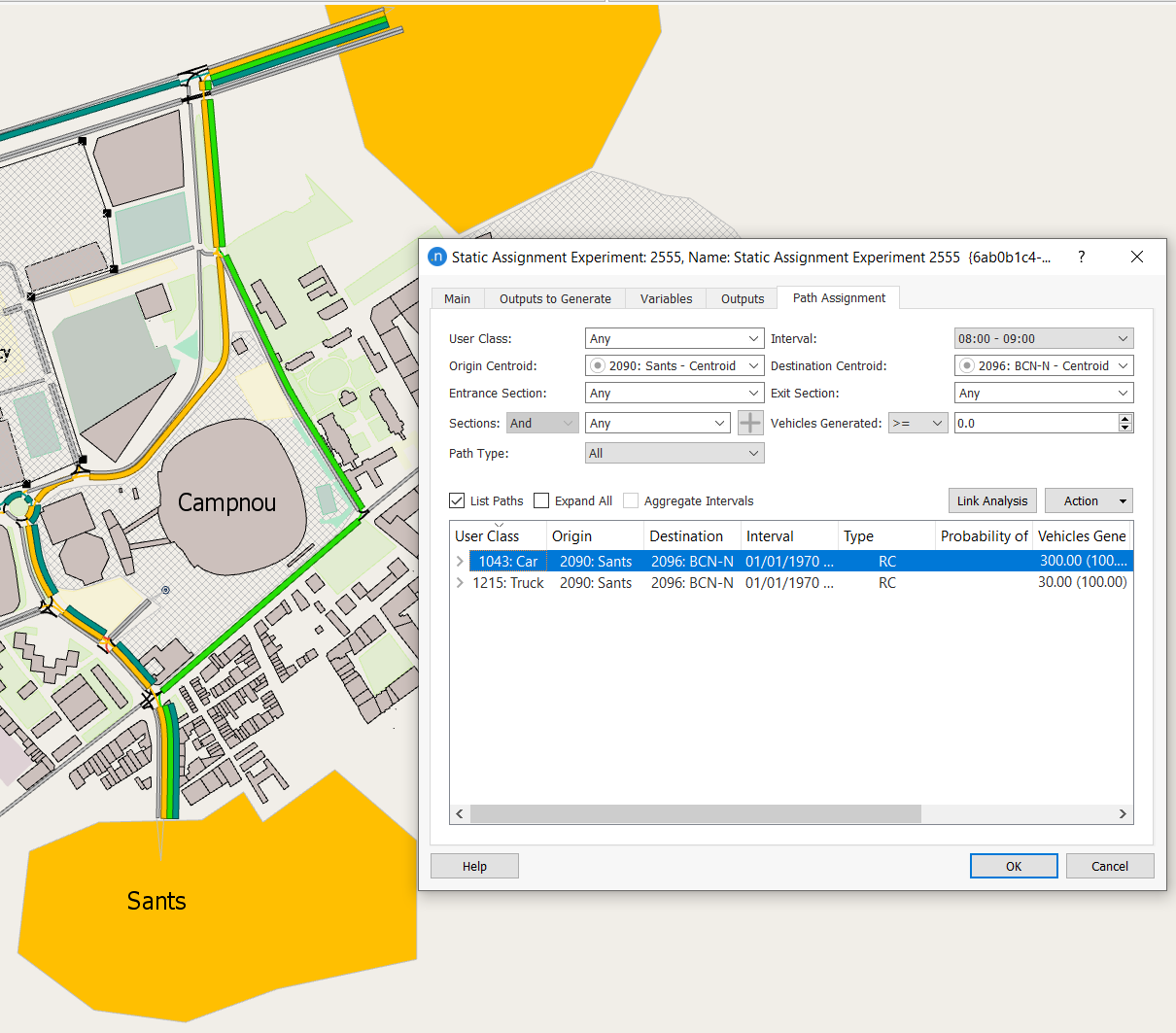
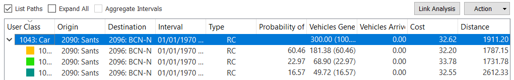
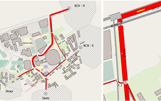
Click the Path Assignment tab to view all the paths used in the assignment by vehicle type.
-
To view specific paths, for Origin Centroid, select Sants and for Destination Centroid, select BCN-N.
-
Tick List Paths to display the paths in the 2D view.
-
Double-click on a path to display more information.
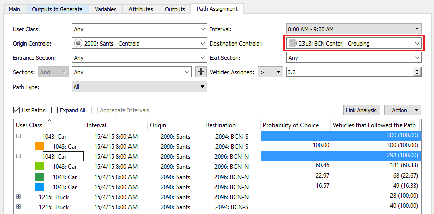
Instead of single centroids, you can use groups of centroids to analyze the paths. These groups are already defined in the network.
-
For Destination Centroid, select BCN Center – Grouping as shown below.
-
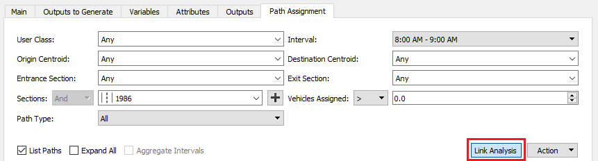
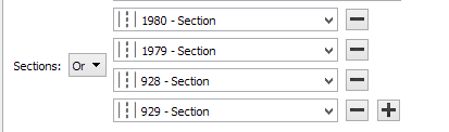
Select a road section from the Sections drop-down list.
-
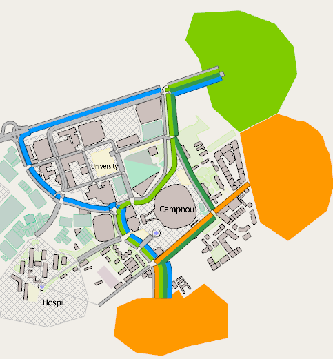
Click Link Analysis to display a map that shows the paths of vehicles that pass through this particular section. The 2D view shows the routes leading to and from that link.
-
Try other selections, filtering by centroid and by user class to better understand the paths chosen by vehicles.
-
To add multiple sections, click the plus (+) button.
-
Select AND or OR to specify how to combine the sections:
- AND analyzes paths which use a stream of sections
- OR has the effect of analyzing with a screenline.
-
To remove sections, click the minus (–) button.
Exercise 2. Adjusting an OD Matrix
In this exercise we will adjust an OD matrix based on real data for the time period. We will use a CSV file that contains detection data for a period of one hour, collected every half hour.
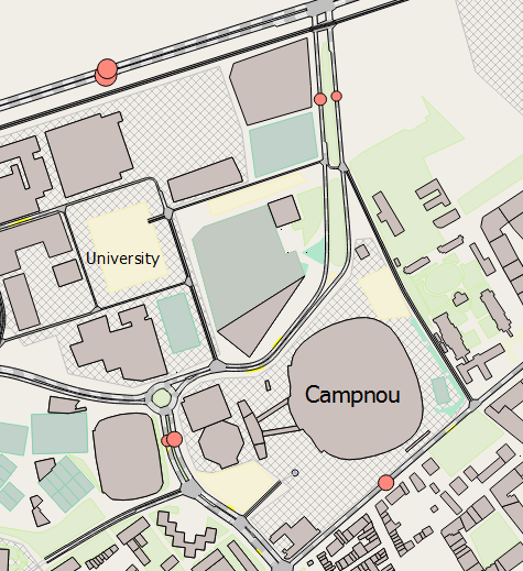
The file contains data from the detectors in the model named d1 to d7. The screenshot below shows the location of the seven detectors.
2.1 Loading the real data set
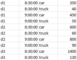
First, we will load the CSV file as our real data set and view its time series. The file is detectors.csv and uses the format: name, time, vehicle, count.
To load the real data set:
-
In the Project folder, right-click Data Analysis > New > Real Data Set to create a new Real Data Set object.
-
Open the real data set and click Add. The following dialog is displayed.
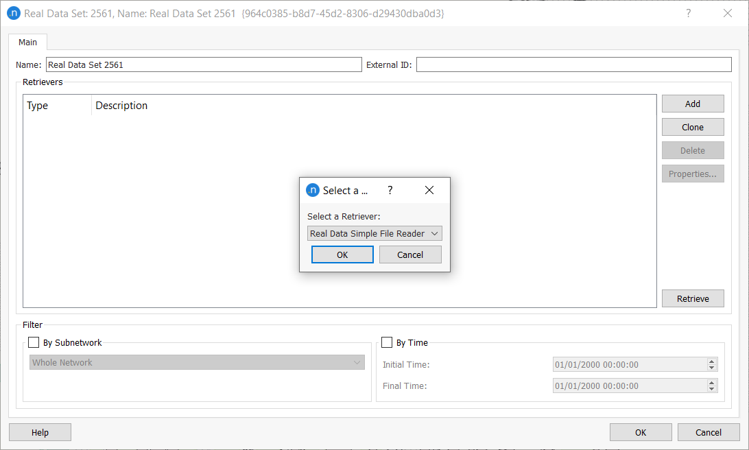
-
Click OK to accept the Real Data Simple File Reader.
-
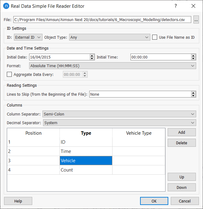
In the Real Data Set dialog, double-click Real Data Simple File Reader in the Retrievers group box. The data reader dialog is displayed. Use the screenshot below as a guide for the next steps.
-
In File, locate the file detectors.csv.
-
Input an Initial Date of 16/04/2015.
-
Click Add four times to add four new items to the Columns group box.
-
For items 3 and 4, double-click in Type and select Vehicle and Count respectively.
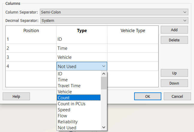
-
Click OK to return to the Real Data Set dialog.
-
Click Retrieve to load the data.
-
To check that the detection data has been correctly loaded, double-click on detector d1 in the 2D view.
-
Click the Time Series tab folder and click Variables.
-
For the Y axis, select Count and Real Data Set.
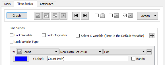
-
Click Graph to view the plot as shown below.
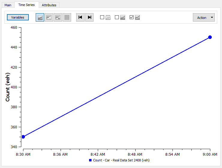
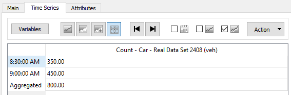
To return to the tabulated figures, click the table icon
 .
.
2.2 Creating the static OD adjustment scenario and experiment
With the real data loaded, we can create the scenario and experiment.
To create the static OD adjustment scenario and experiment:
-
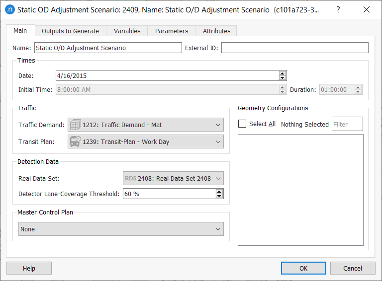
In the Project folder, right-click Scenarios > New Static OD Adjustment Scenario.
-
Open the new scenario and input the parameters shown below.
-
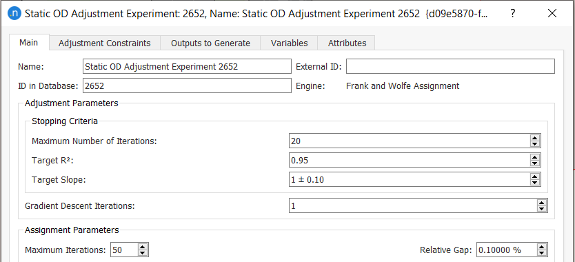
Create a new experiment for the scenario and select the Frank and Wolfe assignment method when prompted.
-
Enter the iteration parameters, using the screenshot below as a guide, and click OK.
-
Right-click the experiment and select Run Static OD Adjustment.
2.3 Viewing the results
When the experiment is completed, the results will be available in the Static OD Adjustment Experiment dialog.
To view the results:
-
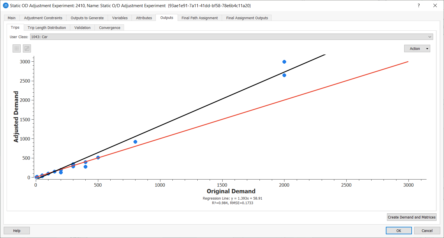
Click the Outputs tab and then the Trips subtab to see original demand vs adjusted demand, as shown below.
-
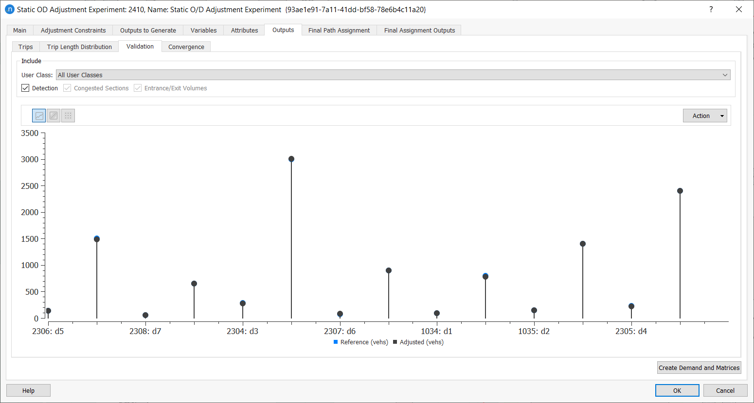
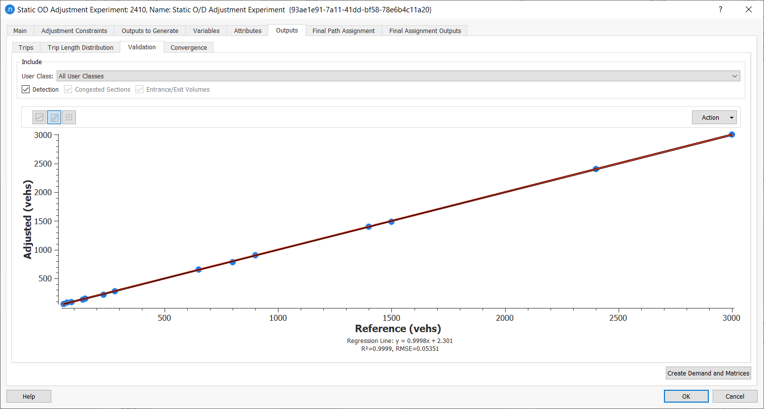
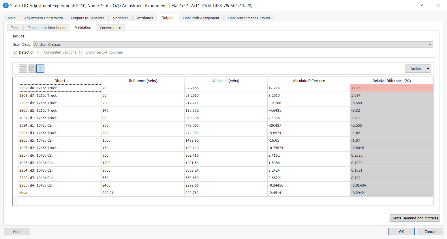
Click the Validation tab to compare the observed counts with the assignment of the adjusted matrices, as shown below (use the nearby icons to view line graph, regression graph, and table).
-
If the validation is satisfactory, generate the matrices and corresponding demand by clicking Create Demand and Matrices. This creates a new traffic demand that contains the adjusted matrices.
-
To use these new matrices, create a new static assignment scenario and assign the new traffic demand to it.
-
Create a new experiment for this scenario.
-
Run the experiment and observe the new flows.
Exercise 3. Calculating Traversal Matrices
In this exercise, we will calculate traversal matrices (car and truck) for a subnetwork, using, initially, the matrix we generated for the whole model. We will then add traffic demand to the subnetwork, using the newly generated matrices.
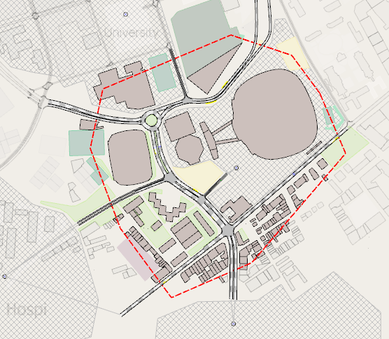
3.1 Creating the subnetwork
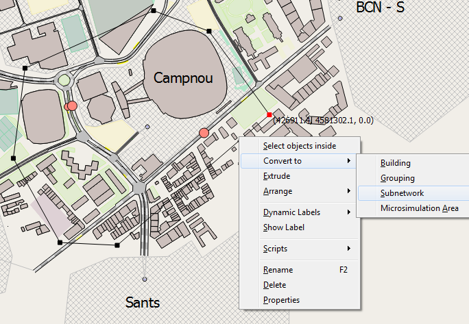
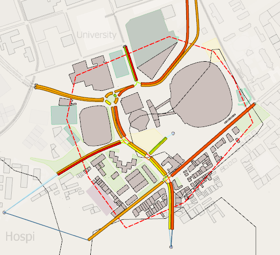
The first step is to create the subnetwork as shown in the screenshot below.
To create the subnetwork:
-
Click
 .
. -
Draw the polygon by clicking its vertices at the required points. To finish and close the polygon, double-click to add the final point.
-
Click on the polygon in the 2D view to highlight it and then right-click Convert to > Subnetwork. A subnetwork object is added to the Subnetworks folder.
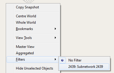
After creating a subnetwork it is helpful to add a filter so that the area outside the subnetwork is drawn in semi-transparent mode.
-
Right-clicking on the 2D view and select Filters > Subnetwork.
3.2 Generating the traversal matrix
To generate the traversal matrix:
-
In the Subnetworks folder, right-click on the new subnetwork and select Generate Static Traversal. The Generate Static Traversal dialog is displayed.
-
For Assignment Experiment, select an available pre-run experiment. This will provided the flow information used to generate the traversal matrix.
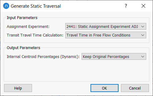
-
Click OK. The traversal matrix (or matrices) will be added to the subnetwork in the Projects folder, inside the Centroid Configurations folder.
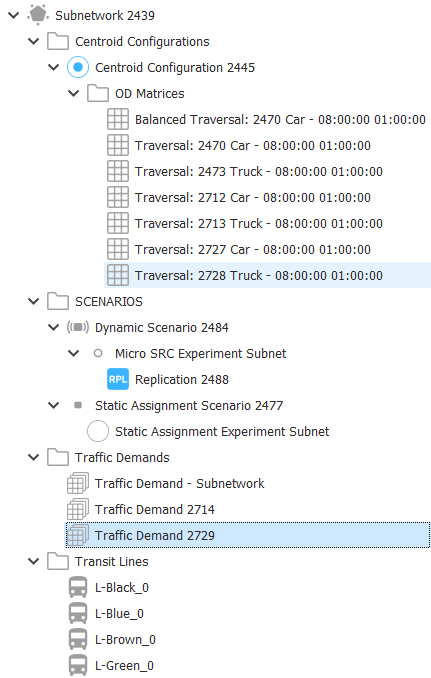
The centroid configuration of the subnetwork is now the active one. An active centroid configuration always appears with its icon highlighted in blue  .
.
All non-graphical objects belonging to this subnetwork (Scenario, Traffic Demand, Path Assignment, etc.) can now be created from its context (right-click) menu. We will do so in Exercise 4. Some objects have already been created and added to the subnetwork, as shown below.
3.3 Running a static assignment scenario
Now we will create and run a static assignment scenario using the new traversal matrices.
To run a static assignment scenario:
-
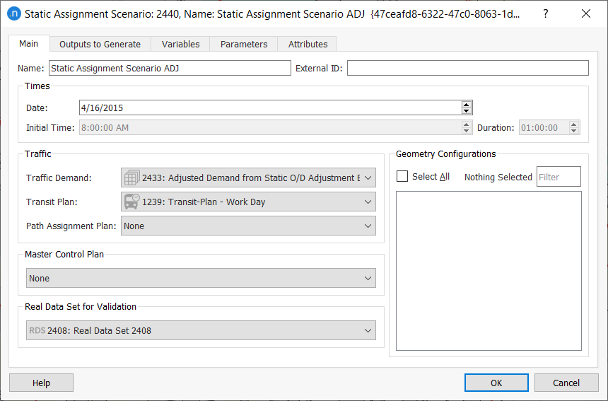
In the Project folder, right-click on the subnetwork and select New > Scenarios > Static Assignment Scenario.
-
Open the new scenario and, for Traffic Demand, select the subnetwork's Traffic Demand object. This contains the traversal matrices.
-
Add a new experiment to the scenario.
-
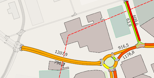
Run the experiment. The visual results of the assignment are shown below.
Exercise 4. Balancing the Matrices
In this concluding exercise, we will use the Furness method to balance the traversal matrices for cars and trucks we generated in Exercise 3. Depending on the source, age, and quality of your demand data in a project, you might need to balance matrices to produce more accurate counts.
Note: Exercise 4.1 relates to the car matrix only. Repeat the same steps for the truck matrix also, so that you have two balanced matrices at the end.
4.1 Copying and balancing the matrix
Because all operations performed on a matrix ‘rewrite’ it when we click OK, we will make a copy of the matrix first.
To copy and balance the matrix:
-
Right-click on Traversal: Car and select Duplicate.
-
Rename the copy Balanced Traversal: Car – 08:00:00 01:00:00.
-
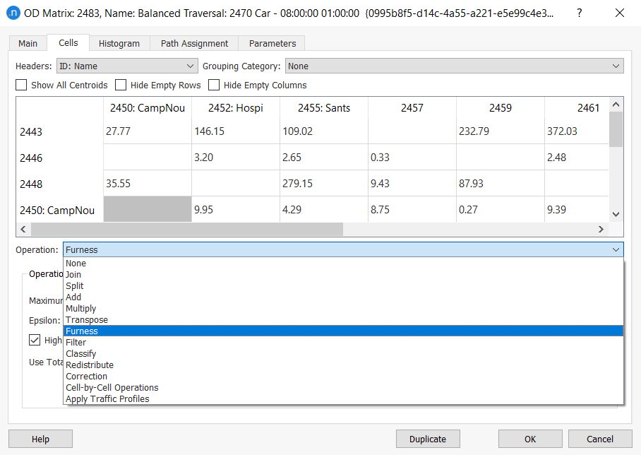
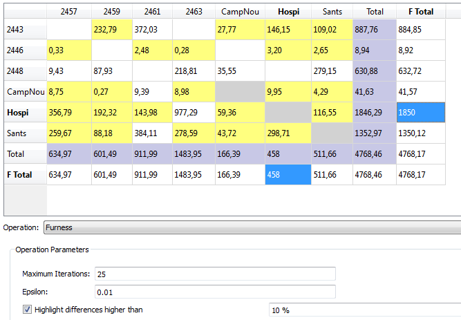
Open the copied matrix and, in the Operation drop-down list, select Furness.
-
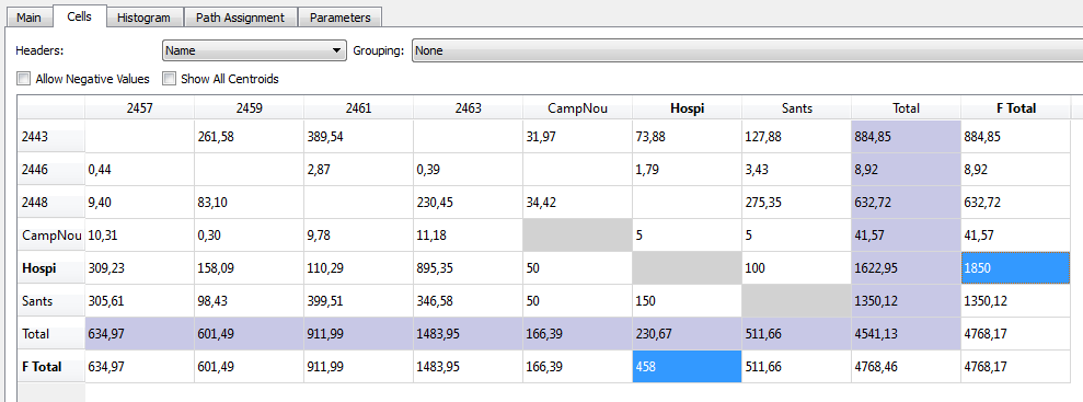
Edit the new totals for the Hospi centroid as shown below. Make sure that the attraction and generation totals match.
-
Click Execute to run the operation. A pop-up confirmation will be displayed when the process is complete. As you can see in the screenshot below, the cells of the matrix have changed so that the F Totals by origins and destinations match the totals we provided.
4.2 Running a simulation with the balanced matrices
To finish this exercise, we will run a simulation of the subnetwork using a new traffic demand with the balanced matrices.
To run a simulation with the balanced matrices:
-
Right-click the subnetwork and select New > Traffic Demand.
-
Open the new Traffic Demand object.
-
Click Add Demand Item and select the balanced car and truck traversal matrices.
-
Click OK.
-
Right-click on the subnetwork and select New > Scenarios > Dynamic Scenario.
-
Open the new scenario and, for Traffic Demand, select the newly created demand.
-
Add a new experiment and a new replication to the scenario.
-
Right-click on the replication and select Run Animated Simulation (Autorun).
Check the simulation to see the results, using the adjusted traversal matrices.