Statistical Methods for Model Validation

The statistical methods and techniques for validating simulation models are clearly explained in many textbooks and specialized papers Law and Kelton 1991, Balci 1998 and Kleijnen 1995. This section demonstrates adaptation of the general process to the problem of validating a dynamic simulation model.

The measured data from the road network should be split into two independent data sets: the data set that will be used to develop and calibrate the model, and a separate data set that will be used in validation. These two data sets can be different data, (i.e. calibrate the mode with flow and turn counts, validate it with journey times) or they can be subsets of the same data (i.e. calibrate the model with one set of flows, validate it with another).

At each step in an iterative validation process, a simulation experiment will be conducted. Each of these simulation experiments will be defined by the data input to the simulation model and the set of values of the model parameters that identify the experiment. These will be adjusted to calibrate the model. The output of the simulation experiment will be a set of simulated values of the variables of interest, in this case the flows measured at each traffic detector in the road network at each sampling interval.

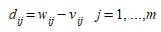
For example: assuming that, in the simulation experiment, the model statistics are gathered every five minutes (the sampling interval) and that the sampled variable is the simulated flow w. Then the output of the simulation model will be characterized by the set of values w~ij~, of the simulated flow at detector i at time j, where index i identifies the detector and index j the sampling interval. If v~ij~ are the corresponding actual measures for detector i at sampling interval j, a typical statistical technique to validate the model would be compare both series of observations to determine if they are close enough. For each detector i the comparison could be based on testing whether the difference over time intervals j (1 to m):

has a mean significantly different from zero or not. This can be determined using the t-statistic:

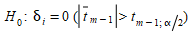
to test for the null hypothesis:

where δ~i~ is the expected value of d~i~ and s~i~ is the standard deviation of d~i~.

• If for δ~i~ = 0 the calculated value t~m-1~ of the Student’s t* distribution is significant to the specified significance level α then we have to conclude that the model is not reproducing the system behavior closely and we therefore have to improve the model.

• If δ~i~ = 0 gives a non-significant t~m-1~* then we conclude that the model is adequately reproducing the system behavior and we can accept the model.

This evaluation will be repeated for each of the n detectors. The model is accepted when all detectors, or a specific subset of detectors depending on the model purposes, pass the test

However, so far as the statistical method is concerned, there are some special considerations to take into account specifically in the case of the traffic simulation analysis (Kleijnen 1995).

1. The statistical procedure assumes identically and independently distributed (i.i.d) observations whereas the actual system measures and the corresponding simulated output for a time series might not follow this assumption. Therefore it would be desirable that at least the m paired (correlated) differences d~i~ = w~ij~ – v~ij~, j=1,…,m are (i.i.d). This can be achieved when the w~ij~ and the v~ij~ are average values of independently replicated experiments.

2. The bigger the sample is, the smaller the critical value is, and this implies that a simulation model has a higher chance of being rejected as the sample grows bigger. Therefore, the t statistics might be significant and yet unimportant if the sample is very large, and the simulation model might be good enough for practical purposes.

These considerations imply that it is unwise to rely on only one type of statistical test for validating the simulation model. An alternative test is to check whether w and v are positively correlated, that is test the significance of the null hypothesis:

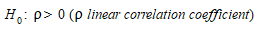
This represents a less stringent validation test accepting that simulated real responses do not necessarily have the same mean and that what is significant is whether they are positively correlated or not. The test can be implemented using the ordinary least squares technique to estimate the regression model:

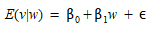
where ε is a random error term.

The test concerns the one-sided hypothesis H~0~: β~1~ ≥ 0 The null hypothesis is rejected and the simulation model accepted if there is strong evidence that the simulated and the real responses are positively correlated. The variance analysis of the regression model is the usual way of implementing this test. This test can be strengthened, becoming equivalent to the first test if this hypothesis is replaced by the composite hypothesis H~0~: β~0~ = 0, and β~1~ = 1 implying that the means of the actual measurements and the simulated responses are identical and when a systems measurement exceeds its mean then the simulated observation exceeds its mean too.

Comparison of the two series v~ij~ and w~ij~ for time intervals j=1,...,m can be achieved with RMSE (Root Mean Square Error) measures, Theil's U or the GEH statistic.

RMSE

If, for detector i the prediction error in time interval j (j=1,...,m) is d~ij~ = w~ij~ – v~ij~, then a common way of estimating the error of the predictions for the detector i is “Root Mean Square Error”.

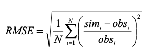
This error estimate has perhaps been the most used in traffic simulation and, although obviously the smaller the value of rms~i~ the better the model, it has quite a significant drawback, as it squares the error, thereby emphasizing large errors.

Theil's U

Thiel's U statistic (Theil 1966) is a measure of association between two series where a value of 0 implies there is no difference between observed and simulated data and a value of 1 implies there is no relationship between the observed and simulated data.

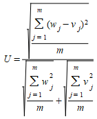
Theil's U can be decomposed to quantify three different types of error.

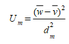
The Bias proportion U~m~ is a measure of the systematic error in the simulation (the nett difference)and is defined as

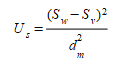
The Variance proportion U~s~ is a measure of the simulation's ability to reproduce the variability in the observed data based on the difference between the standard deviation in the two series and is defined as:

The Covariance proportion U~c~ is a measure of the non systematic error in the simulation or the lack of correlation between the series and is defined as:

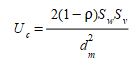
where d^2^~m~ is the average squared forecast error (RMS^2^) S~w~ and S~v~ are the sample standard deviations of the two series and ρ is the sample correlation coefficient between them.

The best forecast is one where U~m~ and U~s~ are close to 0 and U~c~ is close to 1.

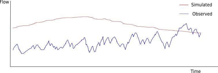
The figure below demonstrates a poor fit for three reasons:

1. The mean for the two series is different (U~m~).
2. The variance in the two series is different (U~s~).
3. The covariance is low (U~c~), the systematic rises and falls in the flows are not correlated.

GEH

The GEH statistic is used to compare traffic volumes. Its name is derived from its inventor Geoffrey E. Havers and is used as an acceptance criterion for travel demand forecasting models by the UK WebTAG guidelines where a set of acceptability thresholds are given; a GEH value under 5 is regarded as a good fit, between 5 and 10 implies the measurement site warrants investigation for error and a value greater than 10 implies a significant and unacceptable error. As the measure is nonlinear, a single set of acceptance thresholds can be specified for a wide range of flow values.

The GEH statistic is defined as:

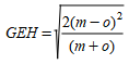
Where m is the modelled hourly flow and o the observed flow.

GEH should be applied to hourly flows only, or flows adjusted to 1 hour values.

In Aimsun Next, the GEH Discrete statistic classifies the GEH value, primarily for display to identify problem areas. The values are:

• GEH < 5: Good fit - value 0.
• GEH 5 - 10 And Observed < Result: Requires investigation, too high - value 1.
• GEH > 10 And Observed < Result: Unacceptable, too high - value 2.
• GEH 5 - 10 And Observed > Result: Requires investigation, too low - value 3.
• GEH > 10 And Observed > Result: Unacceptable, too low - value 4.