Calibration and Validation

In traffic systems, the behavior of the actual system is usually defined in terms of the traffic variables, flows, speeds, occupancies, queue lengths, and so on, which can be measured by traffic detectors at specific locations in the road network. To validate the traffic simulation model, the simulator should be able to emulate the traffic detection process and produce a series of simulated observations. A statistical comparison with the actual measurements is then used to determine whether the desired accuracy in reproducing the system behavior is achieved.

The main components of a traffic microsimulation model are:

• The Road Network
  • The geometric representation of the road traffic network, the road sections, the junctions, and the turning movements.
  • The inclusion of traffic management schemes controlling vehicle speeds, turns allowed, and traffic signal control schemes (phasing, timings, offsets) and the associated roadside detectors, traffic signals, and Variable Message Signs.
• Traffic demand:
  • Input flow patterns at input sections to the road model and turn percentages at intersections
  • Time-sliced OD matrices for each vehicle class
  • The dynamic traffic assignment models which control route choice.
• Individual vehicle behavioral models
  • Car following, lane change, gap acceptance, etc.

All of these components interact and none should be taken in isolation to calibrate and validate a network. However, there is a process in building a model and there are appropriate actions taken to calibrate it at each step. Numerous guidelines exist to aid modelers in meeting the expectations of their stakeholders in building models. Examples include:

• FHWA (USA) Traffic Analysis Toolbox Section 3 in particular covers the use of microsimulation tools
• Transport for London (UK) TfL Modelling Guidelines Which set out modeling and audit guidance for transport assessments.

A review of guidelines can be found in the Multitude Project Case for Guidelines.

This outline of model calibration will discuss 4 stages:

1. Static Checks Build the model of the road network and statically verify it.
2. Dynamic Checks on a running simulation.
3. Travel Demand Estimation.
4. Statistical Comparison with observed data.

Model Build and Static Check

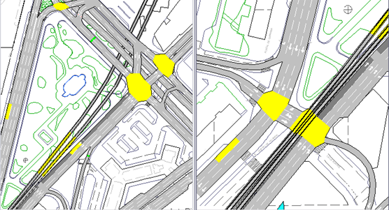
The graphical editor in Aimsun Next has been designed to support the user in building the road network model. Networks can be built by manually superimposing sections and junctions onto a background image imported from a GIS, of a map database (Refer to the Importers and Exporters Section or they can be built by importing directly into Aimsun Next from map data bases such as OpenStreetMap(OSM) which will also import the road characteristics such as the road classifications, the speeds and lanes, and connect the road sections at junctions . Note, however, that while importing directly from OSM might also bring in much more than a graphical background, there is still a requirement to manually check and adjust the imported network.

The figure below illustrates the process of using the graphical editor to build an urban model on the top of a background image.

After the network has been created, the sections correctly configured with road classifications, lane and speed restrictions, and the various artefacts such as VMS, Signals, detectors, and bus stops have been included, the network can be statically checked with the Check and Fix Network Tool. This will validate the network checking for consistency and for any errors such as unconnected sections, conflicting turns, etc. In this way, Aimsun Next will provide a higher level of semi automated network validation than can be achieved by visual inspection from a modeler.

Dynamic Checks

During a simulation, the dynamic checks that can be undertaken are to use the outputs of the replication to observe the number of vehicles lost in the simulation or missing a turn, which is indicative of calibration problems. Similar checks with view modes include looking for areas of heavy braking, once again, with a view mode or to simply observe the simulation in animated mode with background knowledge of the situation on the road.

Estimating Travel Demand

The Travel Demand is arguably the most important component of the model to achieve calibration. Estimating demand from observed data is a significant part of a transport modeling project and Aimsun Next offers some tools to assist with the process. Note though that estimating demand for a small model can be as simple as entering a set of section counts and turn counts into a Traffic State. Alternatively, it might require complex work flows in a multi-level Four Step model with several iterations to generate a robust estimate of demand for multiple user classes in disaggregated matrices. The tools supplied by Aimsun Next to assist in calibrating model demand are described here, the work flow and project management processes which will control how and when they are applied is not.

Matrix Editing

The OD Matrix Editor contains tools to adjust OD matrices. These are documented in the Operations Section for the OD editor and are partly summarized here.

• Split: Creates new matrices by time splitting the original matrix. Typically used in calibration when travel demand varies over time and a single matrix is inadequate,

• Add: Adds trips to the cells of the matrix. Using the selection criteria, this can be used to make manual incremental adjustments to demand to investigate calibration options

• Multiply: Multiplies the trips in the matrix by a given factor to increase or decrease overall demand.

• Transpose: Transposes the matrix or part of it. Typically used to generate a return matrix, i.e transpose the AM commuter matrix to generate the PM matrix, which can be used in the simulation or compared with an existing matrix.

• Furness: Adjusts a matrix after growth factors have been added to some trip ends. Typically to distribute trips if a calibration option requires trip numbers to or from a centroid are varied.

• Correction: This operation will apply the same multiplicative changes to the current matrix that were made from an original matrix to a manipulated matrix. Used in calibration to ensure matrices can be altered consistently if this is appropriate.

Matrix Adjustment

A Static Adjustment Scenario is a procedure for adjusting an a priori OD matrix, using traffic counts. It is used to adjust a matrix derived from demand predictions to agree with traffic observations from the road. The Static Adjustment Scenario contains options to group detectors or to group centroid connections to improve the robustness of the adjustment estimates. These options should be considered when using this scenario.

Detector Location

The Detector Location Tool is a companion tool to the Static Adjustment Scenario. The adjustment process depends on adequate data coverage from the roadside detectors to ensure the majority of trips are observed and the adjustment is not altering trip numbers that are unobserved. The Detector Location Tool analyses the trip coverage and suggests where on street detectors could be placed.

One application would be to create the model and run it with a false demand of one trip between each OD pair to assess the initial routing and with that, apply the Detector Location Tool to guide the data collection exercise.

Departure Adjustment

The Departure Adjustment Scenario is a procedure to create a profiled demand from a static demand. In a microsimulation model or in a mesoscopic simulation, travel demand can be represented at short time intervals ( Typically minutes compared to the ubiquitous 1 hour matrices used in a static assignment) This more accurately reflects the true nature of travel demand which is controlled by factors such as "the school run" or a departure time from employment or an event.

The Departure Adjustment Scenario splits OD matrices into a set of matrices with shorter time intervals and adjusts the demand in each to match the time varying profile of the observed data, taking into account the journey time between the trip departure point and the data observation point. Creating profiled matrices will assist in calibration with data measured at short time intervals, or for example modeling the build up and dispersal of a queue.

Validation

Once a vehicle-based simulation has been run or an average of simulations has been calculated the replication editor, result editor or average editor has data in the Validation folder.

The aim of the Validation folder is to be able to compare the results from the simulation with Real Data defined for the Scenario.

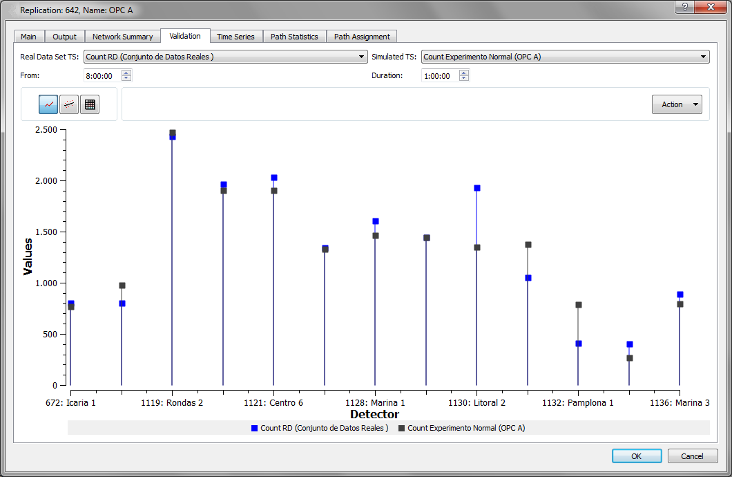
Once the real data set is defined and the simulated data is available, the Validation folder will look like the one in the figure below.

The Real Data Set Time Series and the Simulated Time Series are selected in the drop-down menu and displayed in 3 ways:

• As a graph
• As a regression analysis
• As a table

To display the real data set data vs. the simulated data as a graph, click the graph icon in the figure below.

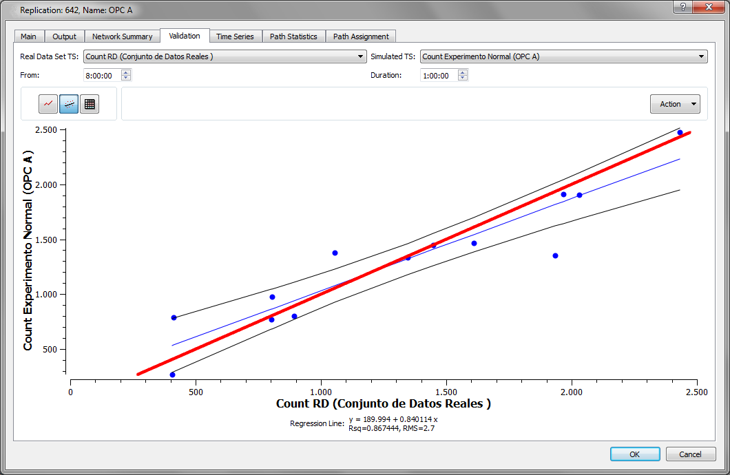
To display a regression of the real data set data vs. the simulated data, click the regression line icon in the figure below. Information about the linear regression line, Rsq (Coefficient of Determination, R square) and RMS is displayed.

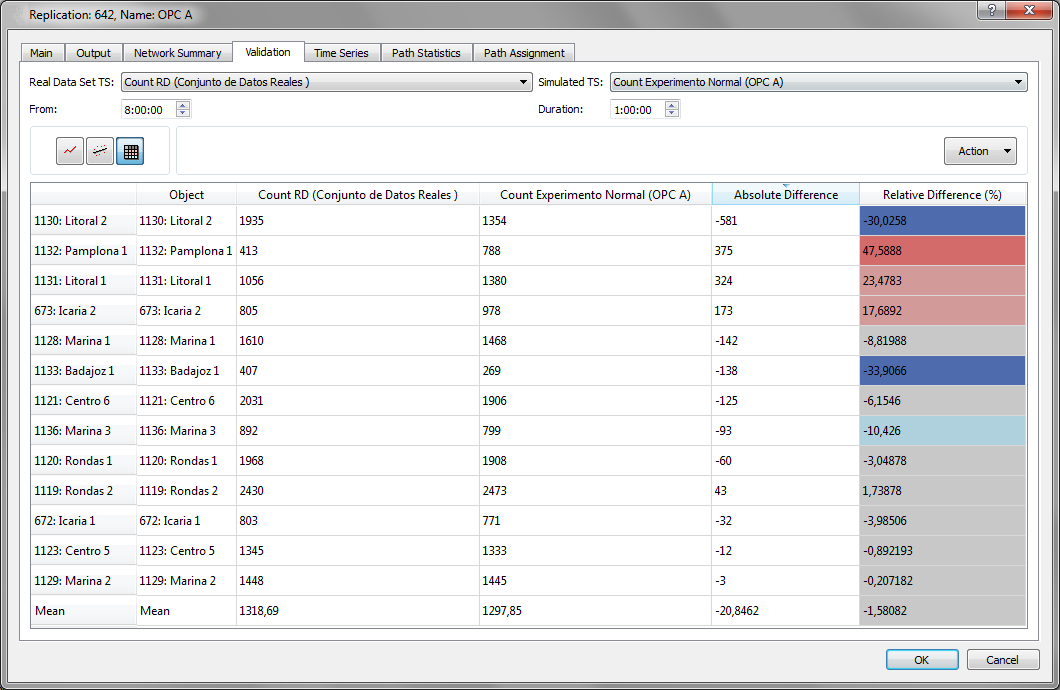
The third option is to display the real data set data vs. the simulation data in a table view. Aimsun Next automatically calculates the absolute difference and relative difference of each pair of values and colors the cells of the relative different depending on its value to give a easily assimilated visual impression of where the main deviations lie.

Additionally to the information displayed in the Validation folder, two other validation statistics can be calculated:

• Theil statistic
• GEH statistic

These statistics are described in more detail in the Statistical Methods for Model Validation section.

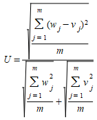
Theil's U

Theil's U statistic is a relative accuracy measure that compares the simulated results (Y) with the real data (X). It is computed as follows

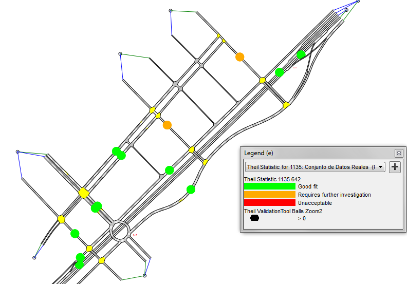
To calculate the Theil statistic for each detector, select the option Action: Calculate Theil. Once selected, two view modes will be automatically created.

Theil Statistic for replication. Where the Theil statistic is calculated for each detector and returns 4 possible values:

• Black - Not applicable. There is no data for the detector.
• Green - Good fit. Theil's U is between 0 and 0.2.
• Orange - Requires further investigation. Theil's U is between 0.2 and 0.7.
• Red - Unacceptable. Theil's U is greater than 0.7.

Discrete Theil Statistic. This is similar to the above view mode with the difference that it includes the sign of the difference between real and simulated measurements.

The Theil's U Statistic view mode is selected in the 2D view as displayed in Figure below.

More detailed outputs from detectors and comparisons with real data are to be found in the Time Series tab for individual detectors.

GEH

The GEH Statistic is used in traffic engineering to compare two sets of traffic data. Although its mathematical form is similar to a chi-squared test, it is not a true statistical test. It is an empirical formula that has proven to be rather useful.

It is defined as:

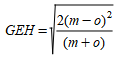
where w and v are the simulated and observed flows respectively.

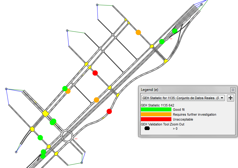
To calculate the GEH statistic for each detector, select the option Action : Calculate GEH. Similar view modes are automatically created as for the Theil’s statistic. GEH bounds are defined using the following ranges:

• 0 - 5: Good fit
• 5 - 10: Requires further investigation
• > 10: Unacceptable

Two types of view modes are automatically created for the GEH statistic. The base view mode GEH Statistic shows the statistic using a simple Red, Amber, Green display.

The Discrete GEH Statistic view mode shows the same data and includes information about the sense of the discrepancy. The values are displayed as above, the legend expands to the following values:

• 0 - 5: Good fit (Green, value 0)
• 5 - 10 And Observed < Result: Requires investigation - Upper (Orange value 1)
• 5 - 10 And Observed > Result: Requires investigation - Lower (Blue value 3)
• > 10 And Observed < Result: Unacceptable - Upper (Red value 2)
• > 10 And Observed > Result: Unacceptable - Lower (Purple value 4)

Detection Patterns

Detection patterns produce a reproducible effect at a detector as if a vehicle of a particular type, length (and possibly transit line) had been present at a given detector at a particular time for a particular duration traveling at a particular speed. Detection Patterns provide for collection of detection events to be stored and replayed in later simulations. Detection patterns are useful for, but not limited to, testing adaptive control plans without applying a traffic demand, thus giving the developer complete control over inputs to a control plan to aid successful debugging.

Detection Templates

Templates can be used when there is a need to reproduce the same or similar detection event many times.