Static OD Adjustment

Matrix adjustment is a procedure that adjusts an existing OD matrix, using traffic counts from detectors, detector stations, and road sections, or turns from nodes or supernodes. The solution algorithm is based on a bi-level model that is solved heuristically by a gradient algorithm, and it includes an assignment at each iteration. For a wider theoretical explanation about matrix adjustment, see Estimation of OD Demand Flows Using Traffic Counts: Matrix Adjustment.

Because the result of a matrix adjustment depends on the quality of data, it is advisable to analyze the quality of the layout of detection data and the quantity of detection sites. You can use the Detector Location tool to find the percentage of demand that is currently intercepted by the current configuration of detectors. See Detector Location for more information.

In Aimsun Next, the adjustment is a multi-user class adjustment. Therefore, we will refer to this procedure as either demand adjustment or OD matrix adjustment.

The adjustment uses two levels of calculations. First, the inner layer runs a static assignment to generate paths and link flows, assigning the current iteration of the OD matrix to the network. The static assignment uses the same parameters (number of iterations and target relative gap for equilibrium assignment, for example) as in a static assignment experiment.

Second, a gradient descent step adjusts the OD matrix using the paths and flows obtained in the static assignment.

The outputs of the adjustment are:

• An adjusted demand and its comparison with the original demand
• A comparison of the trip length distribution between initial and final matrices
• A validation comparing the final assigned flows with the observed data
• A report on convergence as the iterative process runs
• The final assignment results.

A new Traffic Demand can be generated and used as an input for subsequent simulations.

To execute an adjustment, you must create a static OD adjustment scenario and an experiment. The scenario will contain all the input data and the static OD adjustment experiments created for the scenario will contain the parameters for the algorithm.

Static OD Adjustment Scenario

Main tab

On the scenario's Main tab, specify the Traffic Demand to be adjusted. Also, select the Transit Plan to be considered when calculating the assigned volumes, and the Master Control Plan for turn delays, if applicable.

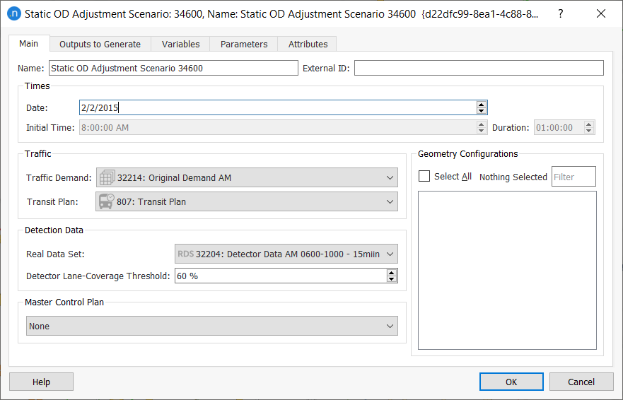
The Real Data Set contains the detection-data time series with observed counts. It can include a value Type per detection named Reliability. This value is considered in the adjustment process as a weight for the difference between observed and assigned data. The larger the Reliability, the more effort the adjustment will make to match that particular pair of values.

Additionally, you can select an adjustment Weight Function on the Adjustment Constraints tab of the static OD adjustment experiment, where it can be given extra factors to multiply the reliabilities. If no reliabilities are set, the software assumes them to be 1.0 by default and the Adjustment Weight values become the final Reliability value.

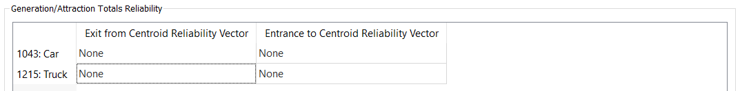
This function applies to values from the detector data for sections, detectors, and turns but not for exits and entrances. You can set additional comparison values for these reliabilities in the Generation/Attraction Totals Reliability group box.

On the Main tab of the scenario, the Detector Lane-Coverage Threshold parameter determines the percentage of lanes a detector and/or detector station should cover in order to be included in the adjustment process.

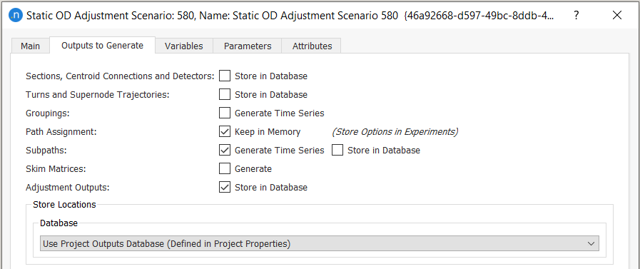
Outputs to Generate tab

On the Outputs to Generate tab you can specify the scenario outputs that you want to generate and store.

Some of the results correspond to the last assignment executed with adjusted matrices. The remaining adjustment results (including the matrices) are saved in a binary ADJ file. If this file is available, the information on the adjustment can be retrieved at any time.

Variables tab

On the Variables tab, you can input the values for any defined variables. To start every gradient descent with the prior matrix instead of the current matrix, add the variable $FIX_PRIOR_MATRIX and set its value to TRUE.

Note: This approach should only be used if complying with the UK Department for Transport (DfT) guidelines.

Parameters tab

If required, set the descriptive parameters from the following drop-down lists:

• Day of the Week
• Season
• Weather
• Event.

Static OD Adjustment Experiment

To create a static OD adjustment experiment, right-click on the static OD adjustment scenario and select New Experiment. In the Experiment Type dialog, select an Assignment Method:

• Frank and Wolfe Assignment
• All or Nothing Assignment
• Incremental Assignment
• MSA Assignment
• Stochastic Assignment.

The assignment method must be specified because the adjustment procedure includes a static assignment at each iteration.

To run the experiment, right-click the experiment and select Run Static OD Adjustment Experiment.

Main tab

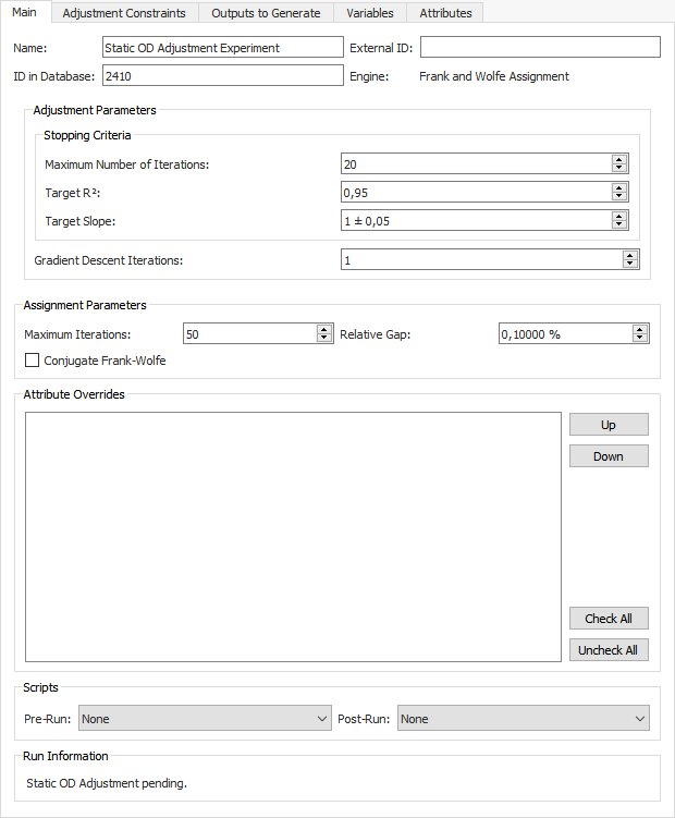
The main tab contains the following groups of parameters:

• Stopping Criteria.

  • Maximum Number of Iterations. At each iteration of the adjustment the process will execute an assignment and use the path percentages obtained from it.

  • Target R². The target R² is a condition that, when met, will stop the adjustment before the maximum number of iterations is achieved. It refers to the quality of the linear regression outputs, which compares observed data with adjusted values.

  • Target Slope. Combined with Target R², this condition stops the adjustment early if the linear regression gives a good R² and a slope close enough to 1 (which is the slope of the reference line where observed for adjusted values).

• Gradient Descent Iterations. For each iteration of the adjustment procedure, this is the number of iterations of the gradient descent method that will be executed without changing the path-choice results (i.e. without executing a new assignment).

• Assignment Parameters. These control the static assignment that takes place at each step of the adjustment procedure. They are documented in the Static Scenarios section and will vary for each assignment type. For example, the All or Nothing (AoN) process requires no parameters whereas the Frank and Wolfe process requires a number of iterations, a relative gap, and the option to tick or untick the Conjugate Frank-Wolfe parameter.

• Attribute Overrides. Tick any existing network attribute overrides to include them in the experiment.

• Scripts. Select Pre-Run and Post-Run scripts to run before and after the experiment.

Run Information is available at the bottom of the folder after the experiment has completed. It gives the execution duration and the version of Aimsun Next used.

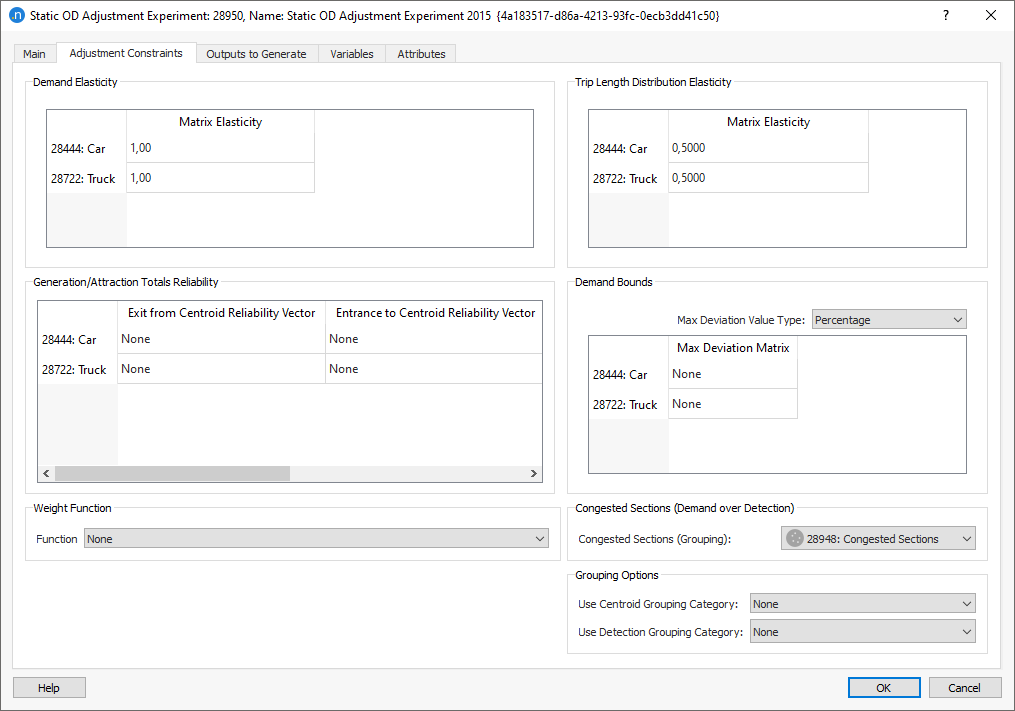
Adjustment Constraints tab

The Adjustment Constraints tab contains the following parameters, which control certain limits of the adjustment procedure.

• Demand Elasticity, per user class. Enter a value between 0.01 and 1.0 to indicate the elasticity of the adjusted matrix with respect to the original matrix. Trips comparison is one of the outputs.

• Trip Length Distribution Elasticity, per user class. Enter a value between 0.01 and 1.0 to indicate the elasticity of the adjusted matrix with respect to the original trip-length distribution. Trip Length Distribution comparison is one of the outputs.

• Generation/Attraction Totals Reliability, per user class. Select the centroid vectors that contain the reliability values of the entrance and exit centroid counts. Leave as None if this parameter is not being used.

• Demand Bounds – Maximum Deviation Matrix, per user class. Select the Max Deviation Value Type (Percentage, Absolute Value, or Factor). Then specify a matrix (with maximum deviation), per user class, to limit the changes in the traffic demand with regard to the original demand. See Adjustment Maximum Deviation for more information.

• Weight Function. Select an Adjustment Weight Function to modify the reliabilities of the section or detector or turn counts. Leave as None if this parameter is not being used.

• Congested Sections (Demand over Detection). When a section is congested, the observed value will be lower than the real demand. To take this into account and to not penalize assignment values higher than the observed congested values, a group of congested sections can be added, if available. For the parameter Congested Sections (Grouping), select a grouping from the drop-down list.

  This means that their observed values will only be used in the calculations while they are higher than the assigned ones. But they will not take part in the adjustment calculations if they are lower than the assigned values. If turn counts are being used, a turn will be considered as congested (and its detection values will be treated the same way) if its origin section is congested.

• Grouping Options

  • Use Centroid Grouping Category. Select a centroid grouping (if available) so that it is considered as a whole in the adjustment procedure, instead of each centroid being adjusted individually. This makes the adjustment less sensitive to route-choice variations.

  • Use Detection Grouping Category. Detector groupings work in the same way as centroid groupings described above. You can set the weight for each detector grouping (the default value is 1.0) and the weight is multiplied by the minimum lane-coverage factor. This is defined as the lane coverage of the detector with the lowest lane coverage that is higher than the detector lane-coverage threshold.

Elasticity

The elasticity values for the matrix and the trip length control how much the values in the adjusted matrix can vary as the adjustment scenario proceeds. An elasticity value close to zero means that the values in the adjusted matrix will be almost unchanged from the prior matrix for that user class. An elasticity value of 1.0 means that no constraint has affected the amount by which the value can be adjusted to match the observed counts (Matrix Elasticity) or the trip length distribution (Trip Length Distribution Elasticity).

Other conditions can then constrain the adjusted value, such as the maximum permitted deviation, which is specified through a matrix of constraints per cell. But the elasticity is a measure of how firmly anchored the adjusted matrix is to the prior matrix.

If the prior OD matrix for one user class is well established and known to be accurate, then a matrix elasticity close to zero would be appropriate. Conversely, if the prior matrix is less accurate – perhaps derived from an older model or where there were known to be subsequent land-use changes – then the matrix would be expected to change more significantly in the adjustment scenario. Therefore an elasticity value closer to 1 would be appropriate.

In both cases, the Max Deviation Matrix can be used to control the variation more precisely.

Adjustment Groupings

You can use Groupings to control the adjustment by merging centroids or by defining groupings for detection screenlines. To select which grouping categories to use, open the static OD adjustment experiment dialog and click the Adjustment Constraints tab. Groupings make the adjustment procedure less sensitive to route choice and increases the reliability of its results.

The following example demonstrates how groupings can be used. Consider the following network with two observed movements: one unobserved – a route choice – and an assigned connection ratio.

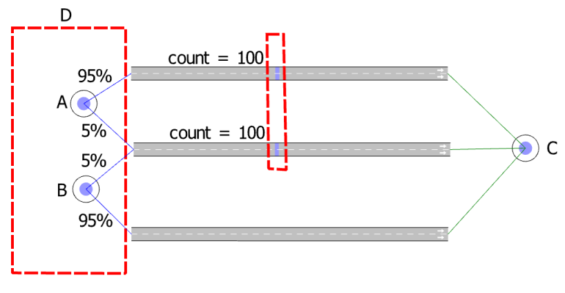
The original matrix is:

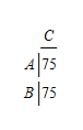
With no groupings, this results in the following system of equations which is fully determined and can readily be solved:

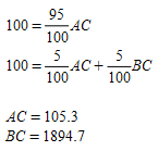
This solution provides a high value for the OD pair BC of almost 2,000 trips. It is very sensitive to the route choice percentage and is largely unobserved. Depending on the model needs and network topology, the following techniques can provide better solutions. Note that "better" does not mean that this gives a better validation result. It is better in the sense of a solution that is less sensitive to route choice changes and is more credible from a traffic-engineering point of view.

Centroid grouping

Centroid groupings aggregate a number of centroids into one aggregated centroid. This reduces the number of variables in the adjustment procedure and can prevent solutions that contain extreme values. In the following example, centroids A and B are grouped into one aggregated centroid called D. The system of equations now has just one variable, DC, and is solved with a least squares method:

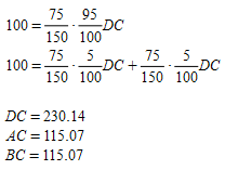
The centroids are then disaggregated and the distribution of the trips inside the aggregated zone is proportional to the original result. In this case the original proportion was 50:50, which is maintained.

Detection grouping

Detection groupings can be used to specify screenlines. This means that several detection locations are aggregated and considered as one detection location. This can be used, for example, if a model has two parallel roads and the route choice between the two is difficult to calibrate. Aggregating the two detectors on this example network will give the following system of equations, which is an under-determined system with many solutions. Running this example in Aimsun Next will give this solution:

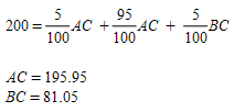
Both techniques discussed above give more reasonable results and are less sensitive to route choice variations.

Additionally, because a detector can belong to more than one detector grouping, it is advisable to tick the option named Exclusive Objects so that each detector belongs to one grouping only. Otherwise, the contribution of a detector will be counted in more than one grouping, which can lead to inconsistent results.

Outputs to Generate tab

The Outputs to Generate tab contains the settings for activating and storing the results of the experiment.

Variables tab

The Variables tab enables you to define values that are not defined in the static OD adjustment scenario dialog, or if different values than those in the scenario are required. Variables specified in the experiment take priority over the same variables in the scenario.

Outputs tab

The Outputs tab contains four subtabs: Trips, Trip Length Distribution, Validation, and Convergence.

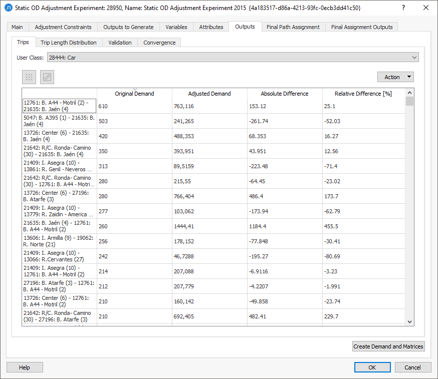
Trips

The adjusted matrices from the experiment are displayed on the Trips subtab. They are presented by User Class (which can be changed) and include Original Demand, Adjusted Demand, Absolute Difference, and the Relative Difference [%]. Click the demand column headings to sort the rows by quantity of demand and difference.

To plot Trips outputs as a regression line, comparing adjusted and original demand, click the graph icon .

To create the new travel demand and its matrices, click Create Demand and Matrices. The new demand and matrices will be stored in the Project folder.

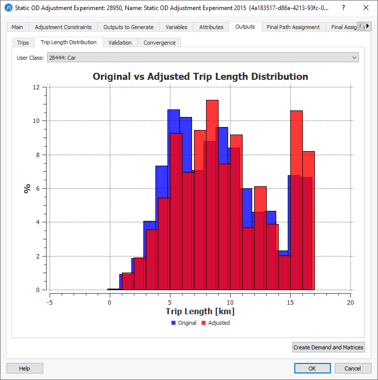
Trip Length Distribution

The adjustment procedure changes the distribution of trips in the simulation. One method of comparison is to study the change in trip length distribution in order to analyze where the changes have occurred.

For example, a significant increase in short trips can indicate that the procedure generated too many "infill" trips between adjacent centroids. In that case, the input constraints and elasticities might need to be reviewed and changed.

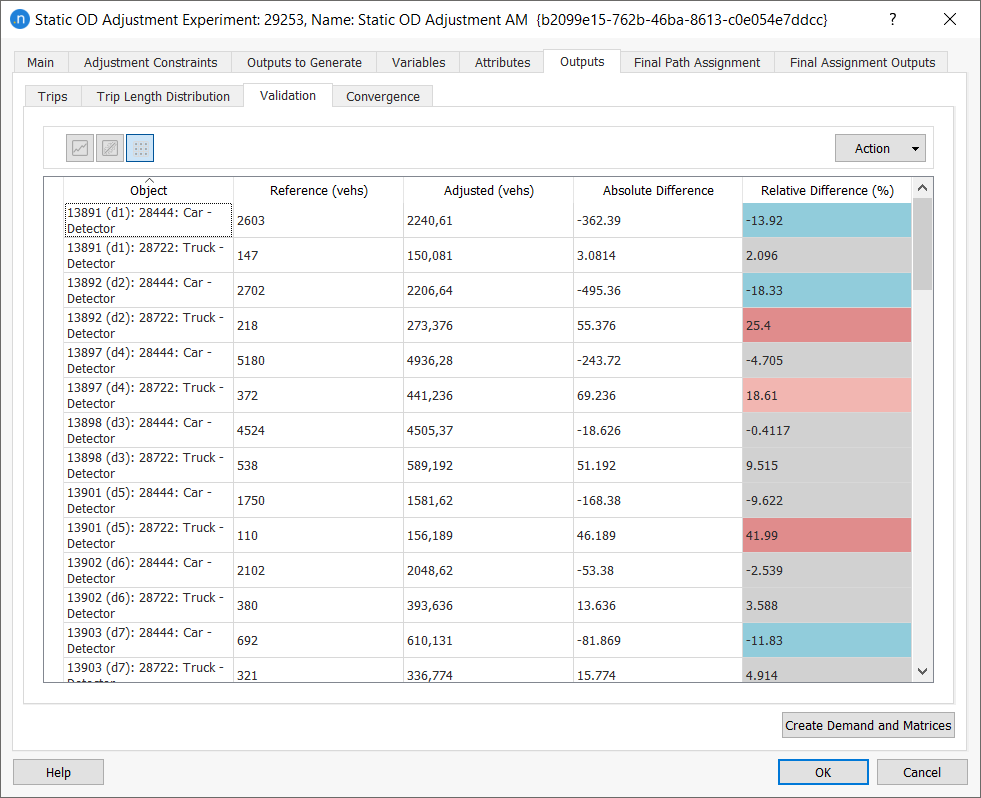
Validation

The Validation subtab compares the results of the adjustment with the RDS. This table will show the

• Detection. This shows the real data set detection data (e.g. section/detector/turn).
• Congested Sections. If congested sections are specified in the scenario they will only appear in this table when the assigned value is still lower than the RDS.
• Entrance/Exit Volumes. This compares the data with the original generated/attracted trips, when these have a reliability associated and have thus been used in the adjustment.

To view the comparison as a regression line, a stick plot, or table, click the appropriate icon .

The Action drop-down menu enables you to Copy Table Data or Copy Graph (Snapshot). A third option, Adjust Limits, enables you to adjust the limits of the stick plot to focus on data in a user-specified range set manually or by reference to an object.

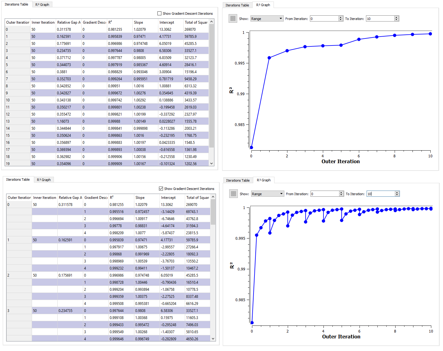
Convergence

The Convergence subtab displays the progress toward the convergence of the R² value and the relative gap of the assignment at each major iteration and, optionally, at each of the intermediate gradient descent iterations.

• Outer Iterations. The number of iterations specified in the experiment for Maximum Number of Iterations.

• Inner Iterations Completed. The number of assignment iterations completed in the experiment. The maximum value is specified in the adjustment experiment Main tab.

• Relative Gap Achieved. The relative gap achieved in the static assignment. This might not be relevant in all static assignment methods. The target value is specified in adjustment experiment Main tab. For more information, see Relative Gap.

• Gradient Descent Iteration (optional). The number of gradient descent iterations completed. The number is specified in the adjustment experiment Main tab.

• R². The measure of the closeness of the fit of modeled flows to observed flows.

• Slope and Intercept. The two values defining the regression line.

• Total of Squares of Errors. The sum of the squares of observed–modeled flows.

The progression of the R² value per iteration can be presented graphically. If it has converged on a value close to 1.0 then the adjustment can be considered complete. If it is still rising toward 1.0 then more iterations might be required. If it is stabilizing at a value much lower than 1.0 then the input matrix, and its constraints, are preventing the adjustment procedure from achieving a satisfactory result.

The screenshots below show the Iterations Table and the R² Graph subtabs with and without the option Show Gradient Descent Iterations selected, where in the adjustment experiment Main tab four gradient descent iterations were specified. Note that only the first 10 iterations are selected for the graph.

Final Path Assignment and Final Assignment Outputs tabs

These two tabs contain the outcome of the last assignment with the adjusted demand. The results are the same as described in Static Assignment Experiment.

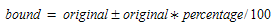
Adjustment Maximum Deviation

In the adjustment procedure, a matrix can be defined (optionally, per user class) using the Contents: Maximum Deviation parameter. This limits the amount of changes the algorithm makes with respect to the original matrix. There are three different value types associated with this parameter: percentage, absolute value, and factor. You can select one of these on the Adjustment Constraints tab of the adjustment experiment.

• Percentage. The values of the specified matrix will be used as a deviation percentage with respect to the original matrix. This results in the following upper and lower bound:

  

• Absolute Value. The values of the specified matrix will be used as an absolute deviation with respect to the original matrix. The absolute value must be positive. This results in the following upper and lower bound:

  

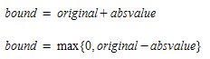
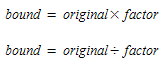
• Factor. The values of the specified matrix will be used as a deviation factor with respect to the original matrix. A value of 0 means Frozen and the value of the deviation factor should be > 1. This results in the following upper and lower bound:

  

In all cases of Max Deviation cells, 0 means Frozen, any positive number is taken as that number, and negative values will be converted to an empty cell, i.e. no deviation is set (or infinite deviation allowed).