Static Scenarios

In a Static Assignment Scenario, flows are assigned to the network using a deterministic algorithm. A Static Assignment does not use individual vehicles, it is oriented about trip volumes and about speed and flows on road sections. It is typically used in wide area models with time periods, used to define the demand in an OD matrix measured in hours, i.e peak, interpeak time periods.

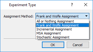
A Static Assignment uses one of five methods to distribute traffic in the network:

The All or Nothing Assignment calculates a single shortest path for each OD pair in free flow conditions (empty network) and assigns the whole OD pair demand to its shortest path. Costs are not updated after assignment, so results will show free-flow costs.

The Incremental Assignment adds iterations to the process. The user will specify the load/unload percentages for each iteration and costs will be updated always after the load and before the unload step. A shortest path with updated costs will be calculated per OD pair at each step.

The MSA Assignment is a method based on Frank and Wolfe but simpler and faster because it skips one calculation, the search for the optimal step lambda, substituting this value by 1/n (being n the iteration number). In general, with a sufficient number of iterations this method will behave well enough and tend toward an equilibrium situation, though this is not assured.

The Equilibrium Traffic Assignment is based on Wardrop's user optimal principle: No user can improve his travel time by changing routes. In Aimsun Next, the Frank and Wolfe algorithm is used to calculate the flows according to this principle. The algorithm is based in a Shortest Paths Algorithm and an ad hoc implementation of a Linear Approximation Algorithm. When using Junction Delay Functions, uniqueness and convergence of solution are compromised. For a wider theoretical explanation about the Assignment, and algorithms used to solve it, refer the section on Static Traffic Assignment: User Equilibrium Models.

The Stochastic Assignment calculates the k-shortest paths for each OD pair and splits the OD pair demand among them according to a Discrete Choice function defined by the user.

The first four are deterministic methods and they are listed in order of complexity. All five are based on the calculation of shortest paths and path percentage usage. These calculations use the cost of the different network elements.

Multi-User Traffic Assignment

In Aimsun Next , matrices are defined for each User Class. A User Class consists of a paired Vehicle Type and Purpose. For example, the trips can be made by the user class: Car – Work. Note the Vehicle Type is mandatory, the Purpose is optional. A Traffic Demand will contain matrices for the different user classes and can contain multiple matrices for each class.

A Multi-User Traffic Assignment consists of a traffic assignment where different types of users are taken simultaneously into account, so that the cost for a user class considers the congestion caused by the volumes produced by the rest of the users. Each user class can perceive a different cost for every section and turn, but the calculation is based on the total volume.

The results correspond to each user class (in vehs), as well as a global assignment result computed by adding the assigned volumes for each vehicle type, additional volumes and the Transit, all of them being considered either in PCU’s (Passenger Car Units) (under the label All (pcu)) or in number of vehicles (when choosing All (veh)). Paths results, however, are not aggregated for All; they are only available per user class.

Static Assignment Scenario Editor

To create a new static assignment scenario, select New > Scenarios > Static Assignment Scenario in the Project Menu. If you are working on a subnetwork, the new scenario can be created from the subnetwork's context menu. The minimum requirement for a static assignment scenario is a base transport network and a traffic demand.

The scenario editor is divided into several tabs which describe what is to be simulated, the outputs to be collected, the variables used to modify the scenario, and some parameters to describe the scenario.

Main Tab

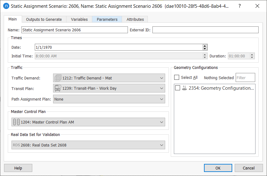
The parameters of the scenario, which will be the defaults for the experiments in this scenario, are:

• The name and external ID of the scenario.
• The simulation time and duration. Note the date is for information and not used by the simulation.
• The Traffic Demand: An OD based Traffic Demand. which can contain one or more OD matrices for one or more user classes.
• A Transit Plan with a set of Transit routes and schedules. The PCU’s corresponding to the volume represented by Transit vehicles along their transit lines will be automatically taken into account in the total volume for all the travel time calculations.
• A Path Assignment Plan with a set of routes derived from a prior static assignment experiment can be selected in MSA and Frank and Wolfe Assignments, so that the Assignment calculations start from this and not from an empty network. Setting a Path Assignment Plan and choosing 1 iteration for the experiment would mean applying the APA file to the demand, with no extra calculation. At least 2 iterations would be needed to calculate new paths and redistribute the demand.
• A Master Control Plan with the signals data used in this scenario. The average cycle times (Calculating Aggregate Control Times) and phases of each turn will then be available for use in Turn Penalty Functions to determine the costs of traversing a signalized junction.
• A Validation Data Set: This is data used to compare simulation outputs with observed data.
• A set of Geometry Configurations: These are the optional variations in the network applied to this scenario.

Outputs to Generate Tab

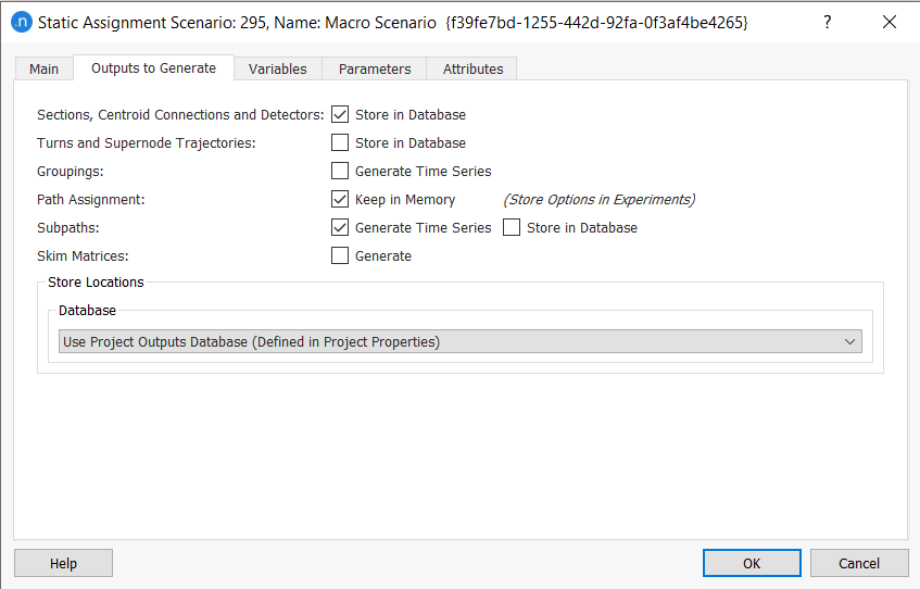
The possible outputs for a static assignment are as follows:

• Flow, assigned volume, and cost data for road sections, centroid connections, and detectors
• Flow, assigned volume, and cost data for junctions and supernode trajectories
• Data for groupings
• Path assignments
• Flow, assigned volume, and cost data for subpaths
• Skim cost matrices.

These can be stored in the project database or in an external database as described in Storing Simulation Results.

For a complete list of output data for static scenarios, see the Output Database Definition topic.

Ticking the Groupings box will recalculate and refresh the groupings statistics (available in the Time Series tab of each group’s dialog) when the static assignment is executed.

The calculation of shortest paths (Path Assignment) is optional: if the Keep in Memory option is ticked, the paths will be explicitly calculated and path outputs will be available after the process, together with other assignment results. Otherwise, no data about the paths used in the assignment will be available, which makes the execution of the scenario faster.

When you tick Path Assignment, you can choose to store the path assignment results in an APA file by selecting a Path Assignment object in the associated experiment's dialog. Statistics for subpaths can also be generated and stored in the database if you tick the options Generate Time Series and Store in Database.

Finally, skim matrices for the generalized cost and distance, as well as for all the Function Components will be calculated and made available in the OD Matrices folder if the Generate checkbox is ticked.

An alternative method of obtaining output matrices is available in the Path Assignment folder in the experiment editor. However, output matrices generated from the experiment will only have values for cells corresponding to non-zero trips, while skim matrices generated from the scenario's Outputs to Generate tab will be full matrices, containing values of the shortest path with 0 trips but taking into account the current costs on the network.

Variables Tab

The variables that will be used in the static assignment are initialized here. Note that these variables can also be defined at the experiment level and in that case, the value will be taken from the experiment. When a simulation starts, the variables are assigned their values by looking first at the experiment and, if no value is defined at that level, then at the scenario.

A variable is an arbitrary string that starts with the dollar sign ($speed and$demand are examples of valid variables).

Static Assignment Experiment Editor

The Static Assignment Experiment is used to run the assignment specified in the scenario with some additional parameters or overridden values for variables. Experiments are created using the "New" option of the scenario context menu.

The experiment context menus is used to run the experiment, it can also be used to:

• Retrieve Static Traffic Assignment Results: This feature reads the assignment results (sections, turns, and convergence data) which were stored in a database when the Static Assignment Experiment was assigned. The database to be read is the one stated in the Static Assignment Scenario editor, Outputs to Generate folder.
• Retrieve Path Assignment Results: This option can be used to read the shortest path information stored in the Path Assignment results file when the Static Assignment Experiment was assigned. The path assignment results file read will be the one stated in the Static Assignment Scenario editor, Outputs to Generate folder.

Depending on the type of static experiment you are running, the wording of the Retrieve [Experiment Name] Results option will differ.

Unloading Data and Results

As a complement to the retrieval options just described, to save memory and enhance performance, there are two options that enable you to unload replication data and path assignment results:

• Unload Static Traffic Assignment Results: Unloads the assignment results that were stored in the database, to save memory and enhance performance.
• Unload Path Assignment Results: Unloads the path statistics and path assignment information from the replication to save memory and enhance performance.

You might find it helpful to select one or both of these options before retrieving data and results from another replication.

Main Tab

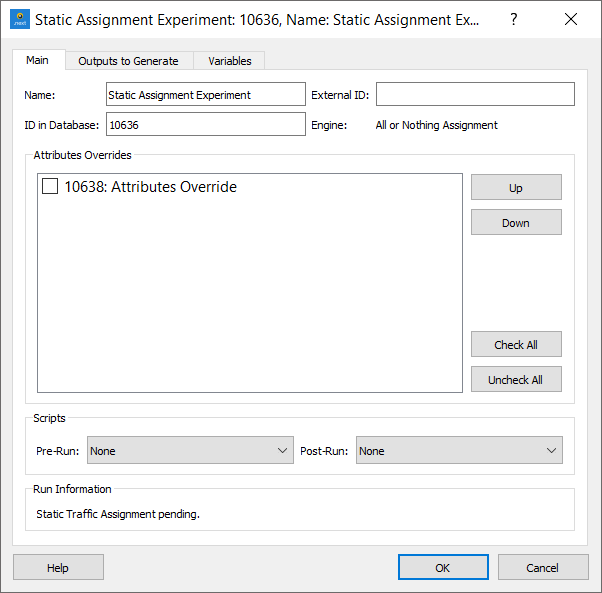
The Static Experiment Editor has different options in the Main Tab depending on the assignment method chosen as the experiment is created.

The parameters common to all methods are:

• Attribute Overrides: The Attribute Overrides for this experiment are selected and the order in which they are applied can be modified.
• Scripts: Scripts can be defined to be run before the execution of an experiment and after the execution of an experiment. These are set in the Pre-Run and Post-Run selectors.

There is a mandatory requirement that both these scripts must contain the following function to check any prerequisite the script might have. This function will return True if the experiment can be run or False if something is missing or invalid; The run will then be cancelled. The signature of the function is:

    def filter( experiment )
    ...
    return True

All or Nothing Assignment

The All or Nothing Assignment model has no additional parameters.

Incremental Assignment

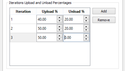
The Incremental Assignment model loads the assignment incrementally. In the example above the first iteration loads 40% of the demand, calculates the travel times on links and unloads 20%. It then loads 50% ( 70% total) and recalculates the link times before unloading 20% and finally assigning the last 50%. Note the total loaded minus the total unloaded must equal 100%.

MSA Assignment

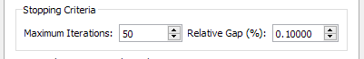
The MSA Assignment process will stop when either the Maximum number of Iterations or the desired Relative Gap is reached.

Frank and Wolfe method

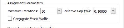
The Frank and Wolfe Assignment model, like the MSA model will stop when either the Maximum number of Iterations or the desired Relative Gap is reached. There is also an option to activate the Conjugate Frank and Wolfe method, a variant to improve convergence (Daneva 2002).

Stochastic Assignment

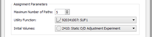
The Stochastic Assignment parameters are:

• The number of k-shortest paths to be calculated.
• The discrete choice function to be used for probabilities calculation, defined as a Stochastic Discrete Choice Function (check the Function Editor for more information).
• The pre-existing loads in the network(optional). Some models might assume there is a capacity drop on links due to traffic that has been separately modeled, these volumes can be pre-loaded here.

Cost Functions

There are three types of Cost Functions which model the macroscopic costs on the network:

• Volume delay functions (VDF) model the generalized cost of the sections and centroid connections.
• Turn penalty functions (TPF) model the primary generalized cost of crossing a turn.
• Junction delay functions (JDF) model the delay caused in a turn, due to the turn volume, the conflicting turn volumes, and the volume on the turn origin section.

The definition of functions in Aimsun Next is done with Python code, so they admit a wide range of possibilities. For example, the user can choose different values for different user classes (depending on the vehicle type or the purpose, etc.) and also define Function Components for specific subfunctions (for example a subfunction calculating the distance in km.) inside the VDF, TPF or JDFs, so that the corresponding new assignment outputs are available. Please check the Functions section for more information on cost functions and function components.

The default template offers a set of VDFs associated with each Road Type in it. The units of the VDFs in the template are minutes, they model the travel time needed to go through a section depending on the volume it has.

The user can add or change the Road Types as well as the VDFs; VDFs can be set by Road Type or defined on a per section basis.

If no VDF is assigned by the user to the centroid connections, they have a default VDF. Users can edit their own functions and assign them to centroid connections.

• Connections to sections or nodes (that is, to the private network) have a default function proportional to its length, with a free flow speed of 1000 km/h (0.06*connection.length3D()/1000). That is quite a low value. Turns between centroid connections and sections are always assigned a zero cost, as they are not editable.
• Connections to Transit Stops or Stations (that is, to the Transit network) have a default function equivalent to walking at 5km/h (12.0*connection.length3D()/1000.0).

The turns in a node also have an associated a default cost (in minutes) for the TPF, which depends on the length and speed of the turn, corresponding to the travel time needed to cross the node in free flow (0.06*turn.length3D()/turn.getSpeed()). Again, users can edit their own functions and assign them to turns.

No Junction Delay Function is assigned by default to turns, so by default, only the travel time needed to cross the junction in free flow is assumed as the turn cost.

Not only the cost functions but also all the parameters they depend on have to be taken care of to get the appropriate results. It is important to check in the definition of each Vehicle Type the value set for the Passenger Car Units (PCUs). Each vehicle has its equivalent value in PCUs in terms of capacity, that is, for example, if the effect of a truck on the network is equivalent to the effect of 2 cars, then trucks should be accounted as 2 PCUs in the calculations.

Cost Function Errors and Constraints

The functions TPF, JDF, and VDF are subject to certain constraints which will trigger errors and the cancellation of dynamic simulations, static assignments, and static adjustments. For more information, see Cost Function Errors and Constraints.

Experiment Outputs to Generate Tab

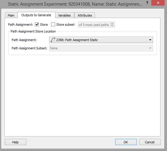
The outputs to generate tab specifies the Path Assignment be to used to store the paths. If only a subset of the paths is to be stored, this can be stored in a separate object. There is an option to store only the first n most used paths, for later use in a dynamic model. The Paths object can be used either to restore the information without recalculating the assignment or with vehicle-based simulators as user defined shortest path trees to simulate dynamically the static equilibrium situation.

Variables Tab

In this tab, the value of the variables that will be used in the simulation can be defined. If they are defined, the value defined here will be used. If they are not defined, the value defined by the Scenario editor under the Scenario Variables tab, will be used.

Running a Static Assignment

A Static Assignment is run from the context menu of the Experiment. The progress is indicated in the Progress Bar. It is always advisable to run the Check and Fix Experiment option before starting a static traffic assignment. This tool is available from the Experiment context menu.

Static Assignment Results

Data Retrieval

The options for Data Retrieval – moving the results from the experiment to the project results database – are located in the context menu of the Static Experiment.The data retrieval options are in the experiment editor. These are:

• Retrieve Static Traffic Assignment results: The data outputs requested for the scenario are loaded to the database specified in the Outputs Tab.
• Retrieve Path Assignment Results: Loads the path statistics and path assignment information from the assignment. In order to load this information an output file must be defined and the related Store option activated.

Depending on the type of static experiment you are running, the wording of the Retrieve [Experiment Name] Results option will differ.

Note: You can also unload this data to save memory and enhance performance; see Unloading Data and Results.

Outputs

The experiment editor for a static assignment will be extended after the experiment has run with an Outputs tab of which contains seven subtabs.

Where appropriate, the data in each subtab can be broken down by user class and if the data in the table is linked to a simulation object, selecting the line in the table moves the main 2D view to that object. Clicking on the header for each column sorts the rows on the contents of that column, then reverses the order. Hence it would be possible for example to identify the turns with the highest flows or the sections with the highest costs.

The Copy button takes a copy of the selected area of the results table and places it on the system clipboard. The data can then be pasted into other applications, e.g. MS Excel, for further processing. The Create Traffic State Button creates new traffic states for the vehicle types in the assignment and inserts them in the Project : Demand Data: Traffic States* list. These can be used to provide demand data for later traffic simulations or exported to signal optimization software such as Synchro.

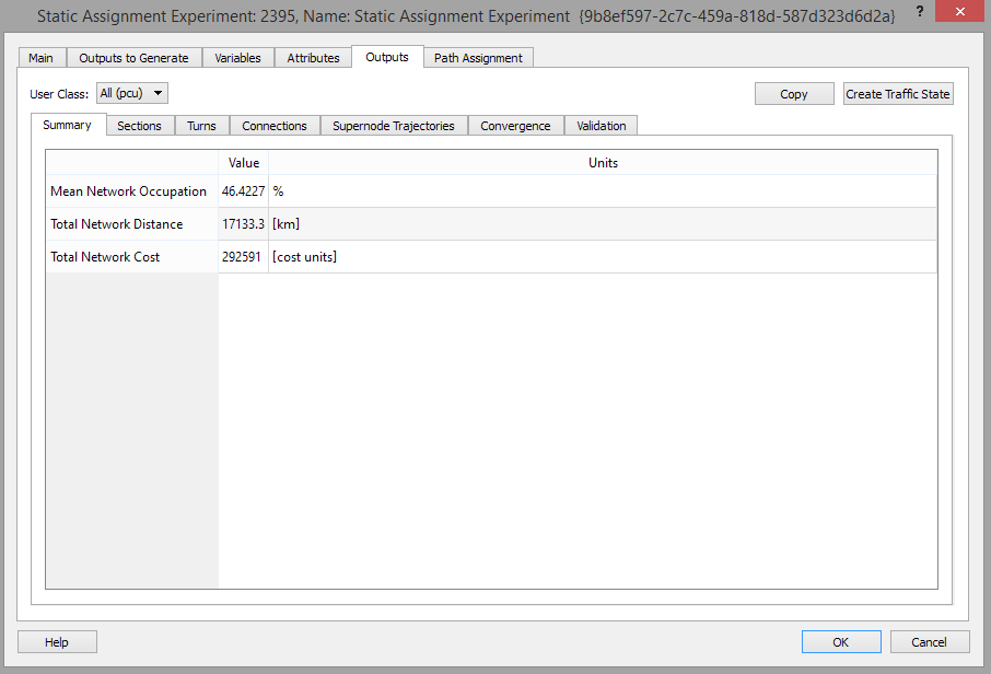
Summary Tab

Summarizes the overall network throughput in mean network occupancy, distance traveled, and cost. These measures do not include centroid connection values. If Function Components have been defined, a global value will be calculated for each one of them (so the previous measures can be obtained including centroid connections by the use of function components).

Sections Tab

Gives the assigned volume, flow, cost, V/C Ratio (an occupancy measure, volume divided by capacity, in percentage) and any Function Components for each section. If the Show Only Entrances box is checked, only entrance sections will be listed; that is sections which are connected to a centroid with a centroid-to-section connection.

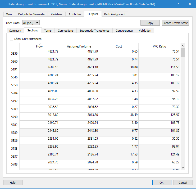
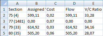
The ‘Copy Data’ button allows copying all the data in the table into a file, as in the example given below.

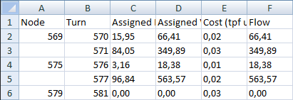
Turns Tab

Gives the assigned volume, cost, and turn percentage for the turns in each node. The Show all Turns button includes the nodes where there was no turn choice( i.e the sole turn has 100% allocated).

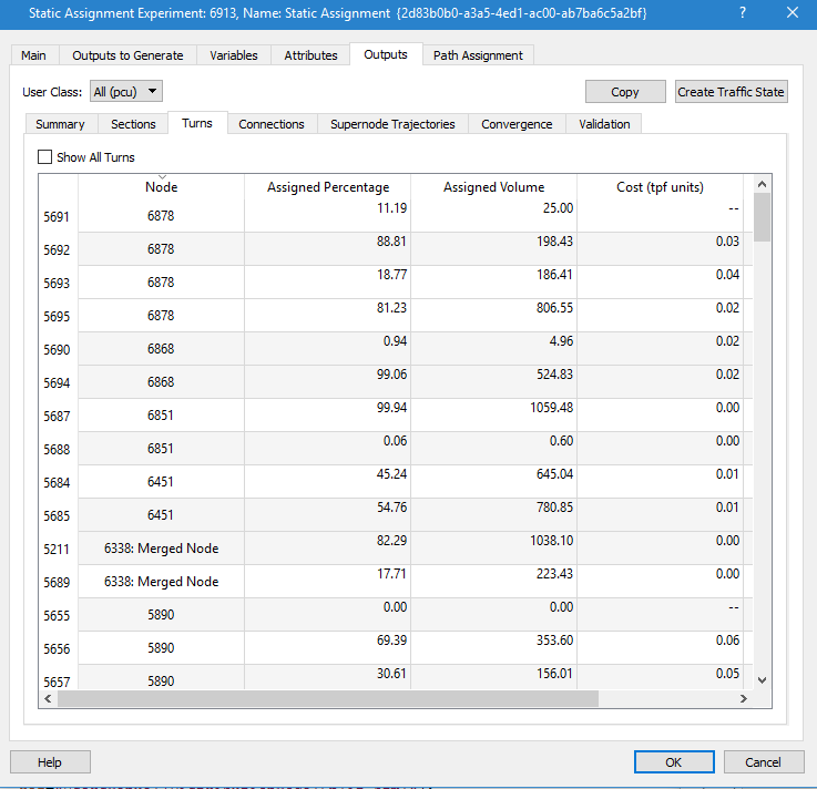
The ‘Copy’ button allows copying the turns results into a file, as in the example given below:

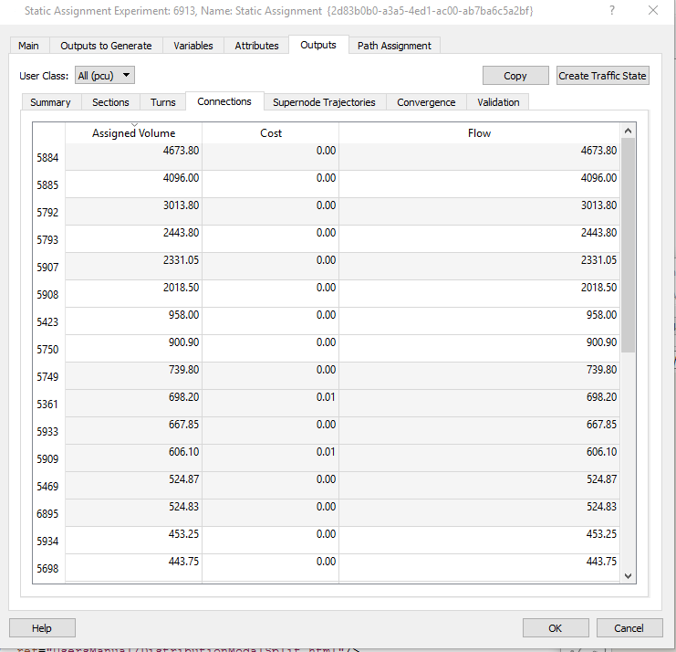
Connections Tab

Gives the assigned volume, flow, and cost for each centroid connection.

Supernode Trajectories Tab

Gives the assigned volume, cost, and turn percentage for the turns in each supernode.

Convergence Tab

This tab summarizes the assignment convergence in tabular and graphical form with the option in the graph to restrict which iterations are shown. For each iteration, the achieved Relative Gap and the Lambda (step length) (when applicable), as well as execution times are listed.

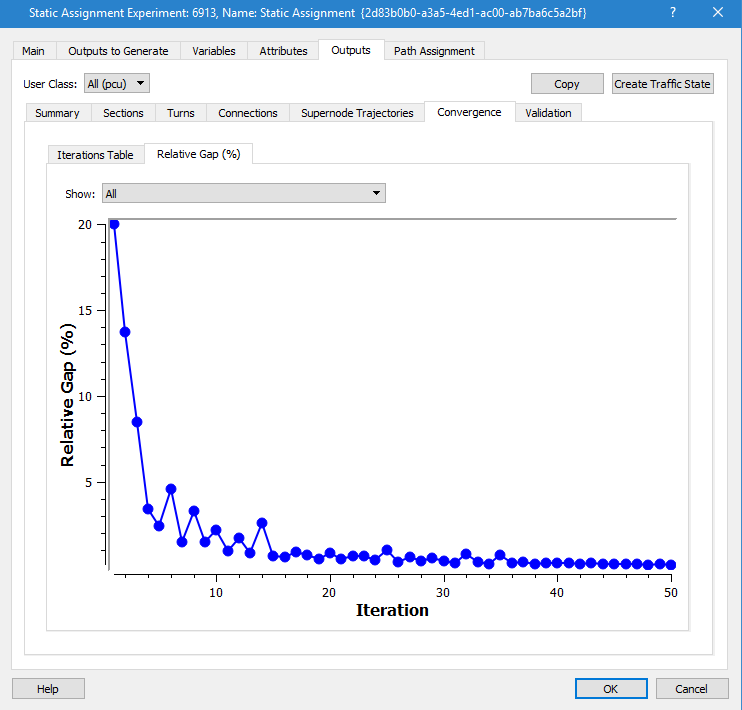
The Relative Gap is a measure of how close the current state of the assignment is to equilibrium (when, for each OD pair, all paths have the same cost). It compares the current costs with the costs on the current shortest paths:

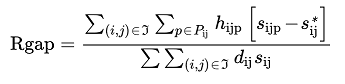
Where:

• h~ijp~ are the trips from origin i to destination j that use path p.
• d~ij~ is the demand (trips) for origin i and destination j.
• s~ijp~ is the cost of path p.
• s~ij~* is the minimum cost of all used paths with origin i and destination j.

Validation Tab

The Validation Tab compares the observed detection data with the flow or volume calculated in the assignment. This uses a Real Data Set for the comparison, that must be loaded and set in the scenario editor Main tab as the Real Data Set for validation.

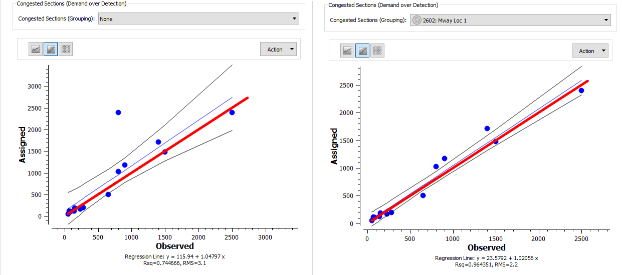
The options in selecting data used in validation are first, to select one or all time series in the real data set (i.e. compare all counts, or just the car counts and truck counts, if the Real Data Set contained those 2 series of counts). The validation calculations can also be configured to omit groups of sections, detectors or turns where the section is congested, i.e. the demand exceeds capacity. Sections can be grouped and each grouping optionally removed from the validation calculations. The effect of omitting measurements from over-congested sections is shown below, helping in the task of focusing on discrepancies on non-congested sites, due to other reasons rather than demand being higher than physical throughput of the network in congested locations.

The validation can be shown as a Graph, a Regression chart or a Table. The options to display the validation data in a static assignment are similar to those used in a dynamic replication.

Validation

Once the Time Series to compare with the Assignment volumes is selected in the Validation folder, there are three different possible representations available: a Graph, a Regression chart or a Table shown in the three figures below.

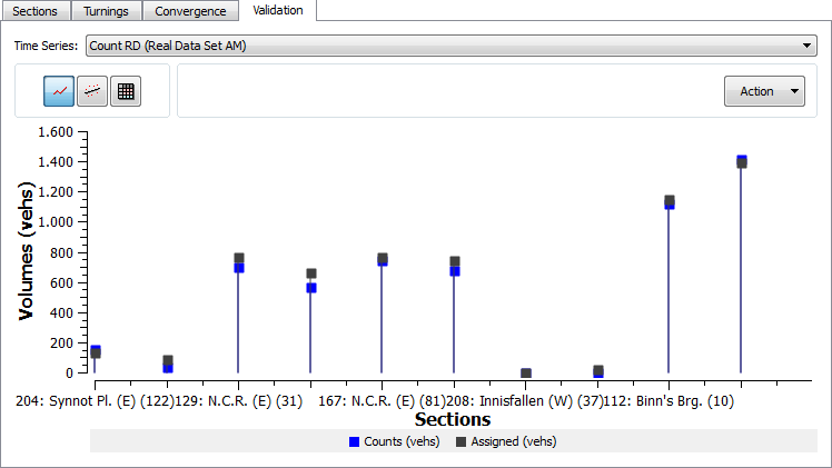
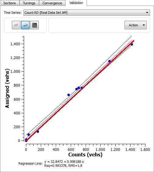
In the Regression graphic, the blue line is the regression line, the black lines are the confidence intervals at 95% and the red line represents the fixed line y = x.

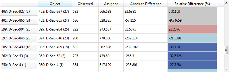
In the Table representation, the observed and assigned volumes or flows are listed, as well as their Absolute Difference and their Relative Difference computed as:

100 * ( (Assigned-Observed)/Max(Assigned, Observed))

Data can be copied into a text file, in the table format with the Copy Date option and the Graph and the Regression Graph can be copied as a picture with the Snapshot option. The limits of the Graph can be set in the Adjust Limits option.

Graphical assignment results

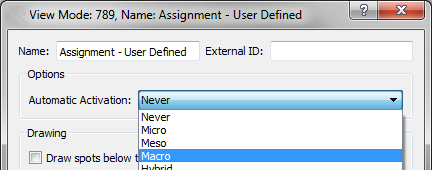
The graphical representation used to show the assignment results in the Outputs folder is defined in the "Assigned Volume" View Mode.

Aimsun Next has a default View Mode for Assignment results, but any of the view modes in the model can be set as the default for showing assignment results by setting the view mode Automatic Activation field to Macro in the view mode’s editor.

The figure below shows an example of graphical assignment results.

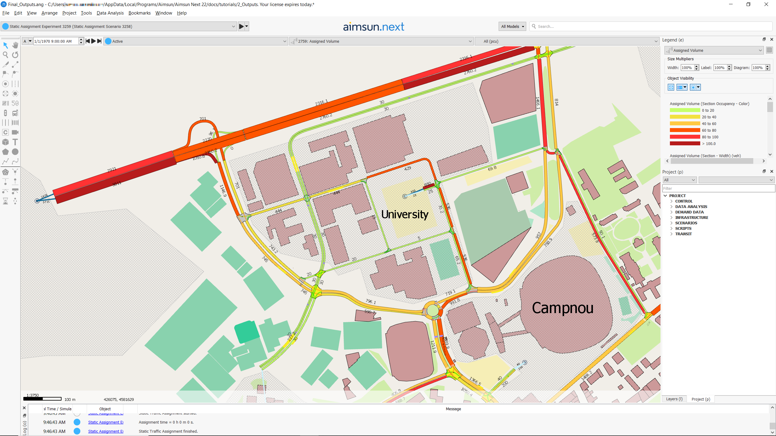
The View Styles included in the Assigned Volume View Mode are:

• Styles for the width of each section, proportional to its volume.
• Styles for the labels of the assigned volumes.
• Styles to hide section objects and nodes.
• Styles for coloring objects based on the volume/capacity percentage (occupancy). By default, a color ramp with six different intervals from green to red is used for sections, and a color ramp in blue tones is used for centroid connections.

Creation of a Traffic State from Assignment results

The section volumes and turn percentages from the assignment can be used to generate a Traffic State with the “Create Traffic State” button in the Outputs folder in the Static Assignment experiment editor .Traffic States for each of the user classes in the demand will be created in the Project window, Traffic States folder.

Path Assignment Tab

The Path Assignment Tab is only shown if the Path Assignment calculation is Activated in the Outputs to Generate folder of the Static Assignment Scenario, and it is available for all user classes except for the aggregated All. It is described in the Path Analysis section and its usage is the same for static and dynamic scenarios.