Modeling Travel Demand

Note about licenses:

These exercises require a license for Aimsun Next Expert or the Pro TDM Edition.

• Exercise 1. Running a Generation/Attraction Experiment
• Exercise 2. Running a Trip Distribution
• Exercise 3. Running a Modal Split
• Exercise 4a. Running a Static Assignment
• Exercise 4b. Running a Transit Assignment
• Exercise 5. Running a Four-Step Model Experiment

Introduction

In these exercises we will look at Aimsun Next's transport planning and demand modeling tools, whose combination will culminate in us running a four-step model.

A four-step model uses trips aggregated by transport zone and the four steps involved are:

1. Generation/attraction: This step determines which trips originate and terminate in each zone, based on the population and land use of each zone.
2. Distribution: This step matches trip origins and trip destinations.
3. Modal split: This step estimates the mode choice that travelers will use for these trips, allocating trips to private transport (vehicles), bicycles, or transit (passengers).
4. Assignment: The fourth step introduces the demand into the transport network and evaluates travel times and costs. In this tutorial, Exercise 4 is split into a (private) and b (transit) assignment.

We will start by preparing and running a generation/attraction (G/A) experiment to create G/A vectors using land-use and travel-behavior data (Exercise 1).

We will then run a trip distribution and a modal split experiment to create OD matrices and assign this demand to the network (Exercises 2, 3, 4a, and 4b).

Finally, we will run a four-step model experiment to link all these processes and their outputs together (Exercise 5).

The backup copies of the files related to this exercise are in [Aimsun_Next_Installation_Folder]/docs/tutorials/9_Travel_Demand_Modelling.

Exercise 1. Running a Generation/Attraction (G/A) Experiment

Data inputs and parameters relevant to this exercise

• Centroids
• Land use data set attributes
• Land use data sets
• G/A area types
• Time periods
• Transportation modes
• Trip purposes and balancing method
• Centroids balancing/non-balancing
• External trips data

In Aimsun Next, open the file Initial_Travel_Demand_Modelling.ang. This network file already contains most of the data needed to run a G/A experiment. Take a look at the available data in the Project window folders; we will complete the data before creating the G/A scenario and experiment.

1.1 Getting familiar with G/A Data

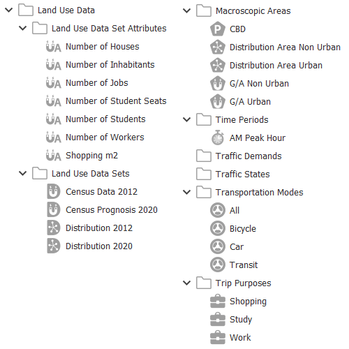
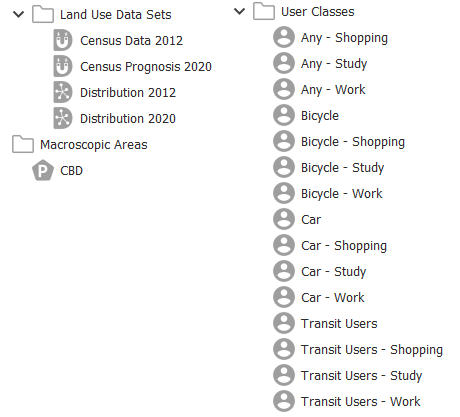
In the Project window, locate and explore the predefined project data: Transportation Modes, Time Periods, and Trip Purposes. Then find the data under the folder Land Use Data, which includes Land Use Data Sets and Land Use Data Set Attributes.

The Generation/Attraction Areas are contained in the Macroscopic Areas folder. Note that the areas are grouped by type name, being Distribution and Modal Split Areas, Generation/Attraction Areas, and Parking Areas.

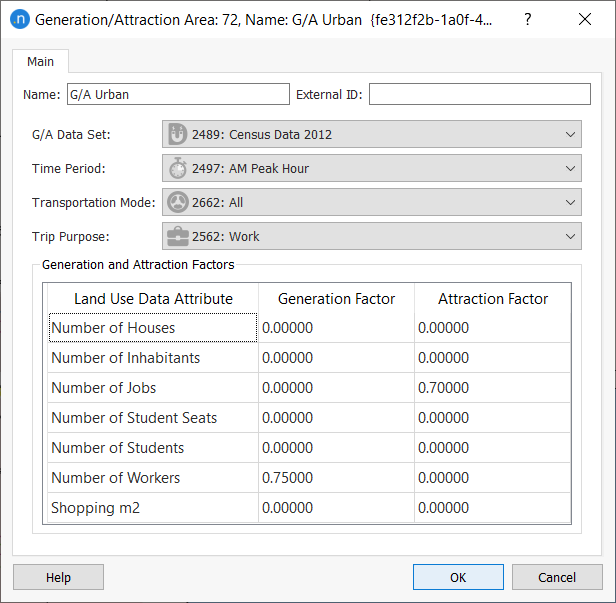
Double-click on any of the objects to see their parameters. For example, for the Generation/Attraction Area G/A Urban, the G/A factors are already defined for the Time Period: AM Peak Hour and the Transportation Mode: All.

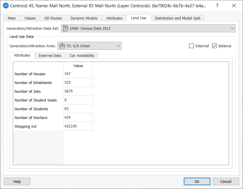
Now double-click on any centroid and click on the Land Use tab:

Some information is already present (Data Set, Generation/Attraction Area, External Data where applicable, and the Balance box is ticked) but the socioeconomic values are all currently 0 and must be added in this exercise.

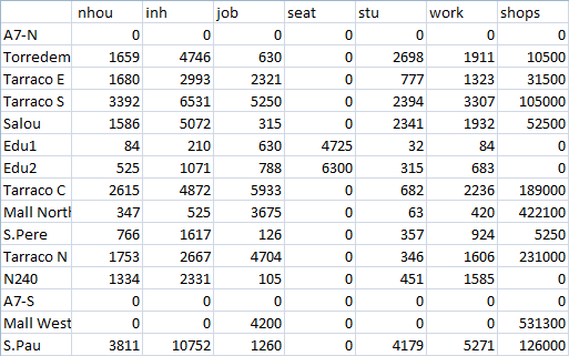
In the same folder as the ANG file, there is a text file containing the data for the data set named Census Data 2012 (CensusData2012.txt). Here is a screenshot of its contents:

To add the socioeconomic values:

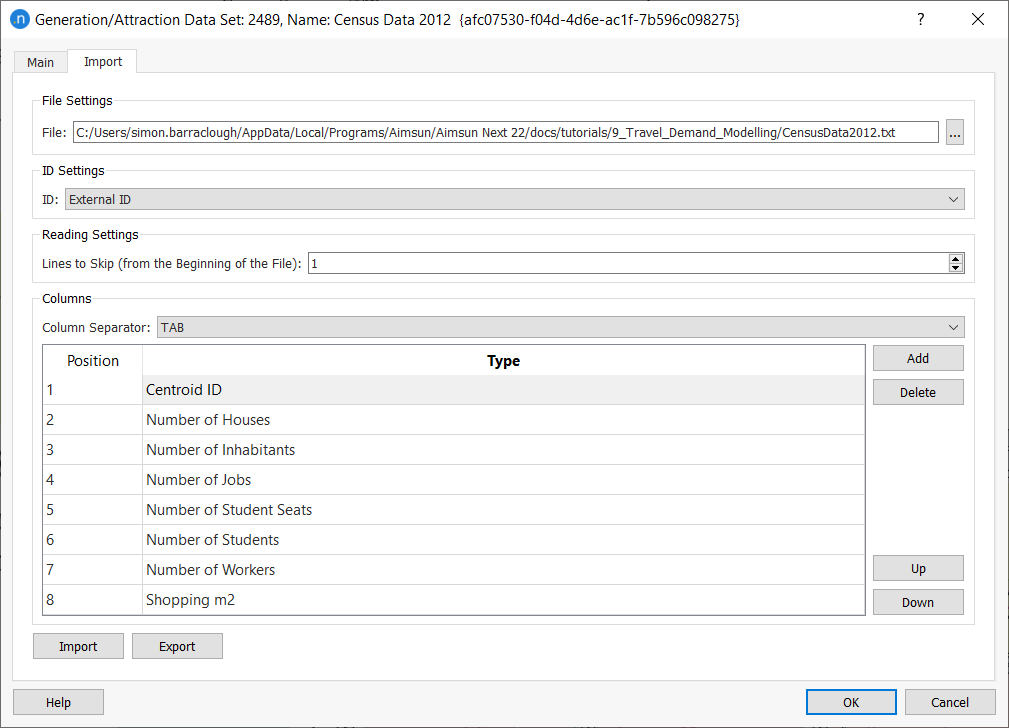
1. Open the data set Census Data 2012.
2. Click on the Import tab.
3. In File Settings, locate the data file CensusData2012.txt.
4. For ID Settings, select External ID.
5. In Lines to Skip, enter 1 (to skip the first, header, line of the TXT file).
6. For Column Separator, select TAB.
7. Click Add eight times to add eight new data rows.

8. Complete the rows as shown below (you can select Type from drop-down menus in the relevant cells).

   
   

9. Click Import to import the data from the TXT file.

10. Check the centroid again to verify that the data is now present):

    
    

    Now we can create a view mode and a view style to visualize some of the data. If you need a reminder about creating view modes and style, see the earlier tutorial Viewing Microscopic Outputs.

11. Create them and define them as illustrated in the next two screenshots:

    
    

    
    

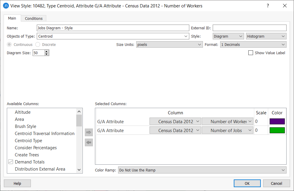
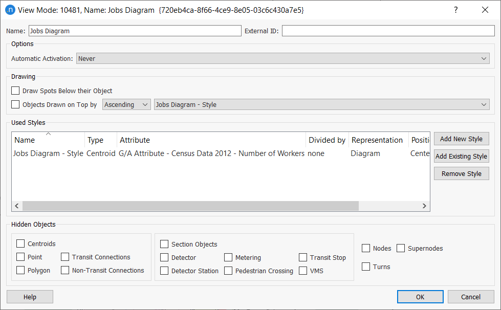
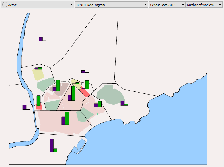
12. Apply them to the view. You should see the histograms in the 2D view as shown below.

    
    

1.2 Running the G/A Experiment

To add the G/A scenario and run the experiment:

1. In the Project window, right-click Scenarios > New > Generation/Attraction Scenario.

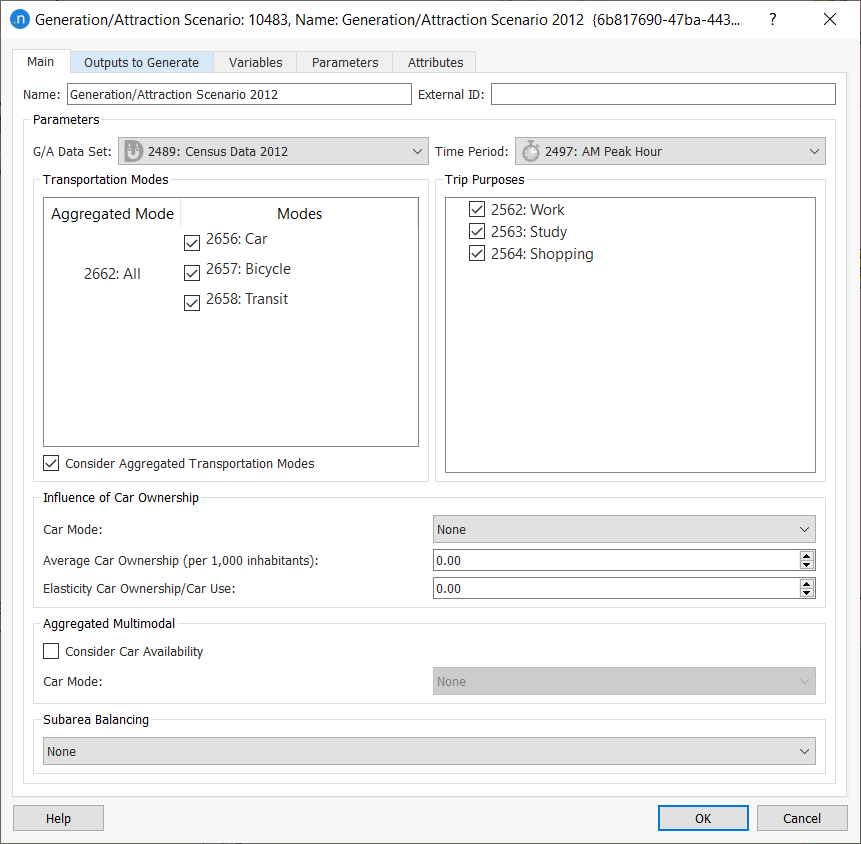
2. Complete the parameters as shown below:

   
   

3. On the Outputs to Generate tab, tick Store in Database so that results can be retrieved later.

4. Click OK to save the scenario.
5. Right-click on the scenario and select New Experiment.
6. Right-click on the experiment and select Run Generation/Attraction. The dialog with summary results is displayed when the experiment finishes.

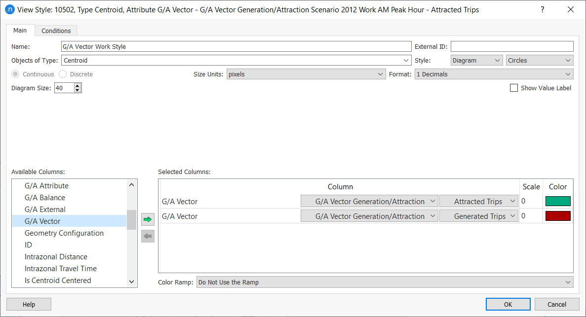
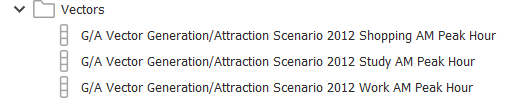
7. Click Generate Vectors to create the G/A vectors. These will appear in a new subfolder called Vectors inside the centroid configuration folder in the Project window. These vectors are the outputs of the process:

   
   

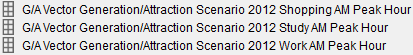
8. Double-click a vector to view its parameters:

   
   

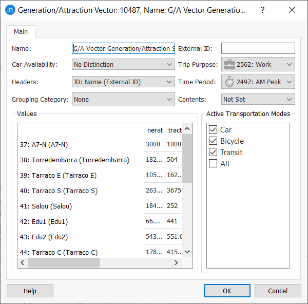
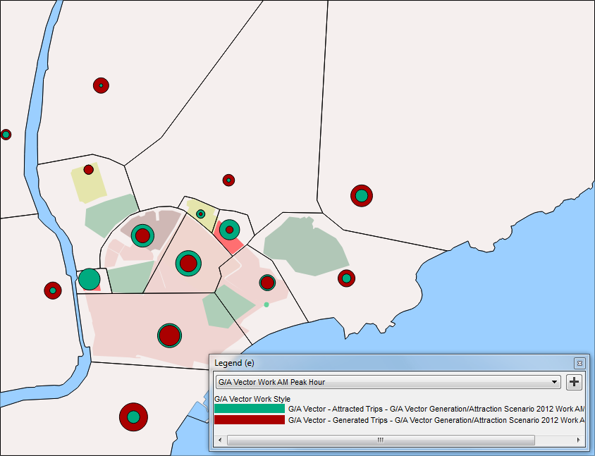
9. Define a new view mode and view style to visualize one of these vectors in the network. In this case, for example, select Style: Diagram and Circles.

   
   

10. Apply them to the view, as pictured below.

    
    

Exercise 2. Running a Trip Distribution

Data inputs relevant to this exercise

• Centroids
• Distribution and modal split data sets
• Distribution and modal split area types
• Parking area types
• Time periods
• Transportation modes
• Trip purposes
• Skim matrices
• Distribution functions

In this exercise, we will look at the data needed for a trip distribution experiment, which will obtain a preliminary estimate of the travel demand.

Take a look at the data required for distribution: Distribution sets, User Classes, Macroscopic Area, Functions, G/A Vectors, and optionally, Skim Matrices containing costs.

There is also centroid-specific data in the Distribution and Modal Split tab of a centroid dialog (see below).

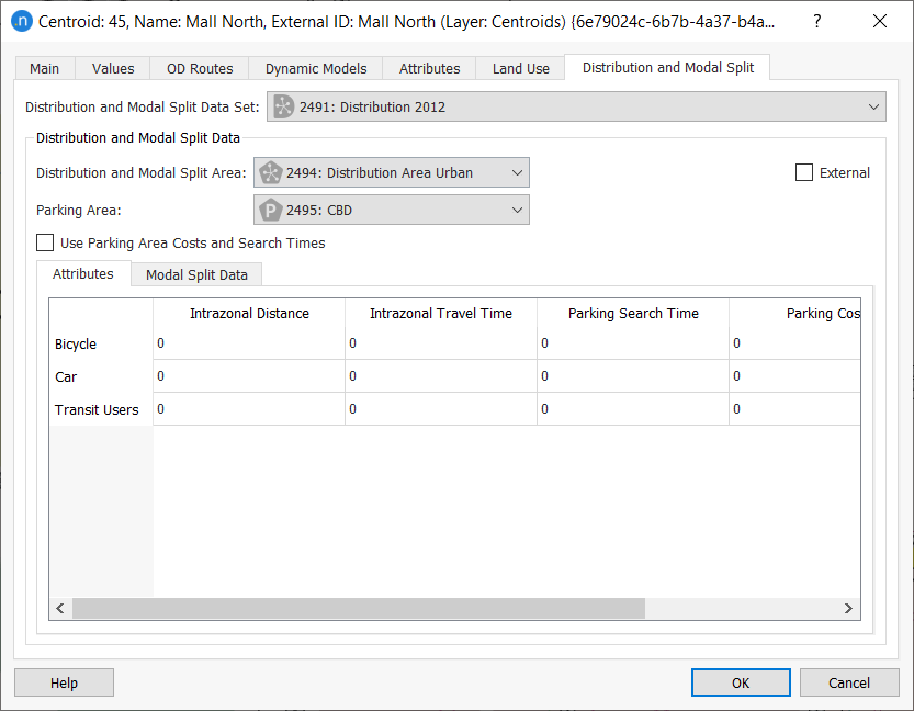
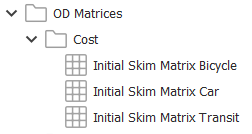
If a set of skim matrices is not available, at this point we would usually run some assignment experiments to obtain preliminary estimates of the travel costs between each OD pair in each mode. In this exercise, however, we already have some initial skim matrices so we can omit this step. You will find these skim matrices in the Project folder here:

To run a distribution scenario and experiment:

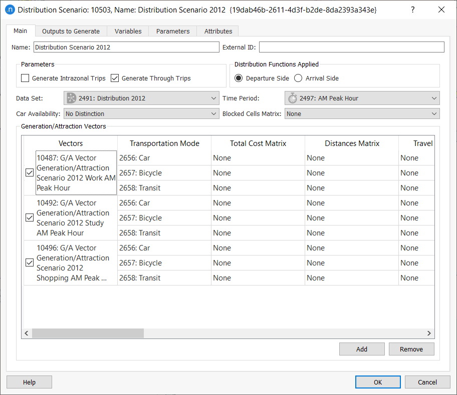
1. Select Scenarios > New > Distribution Scenario and define the parameters as follows:

   
   

2. Right-click on the scenario and select New Experiment.

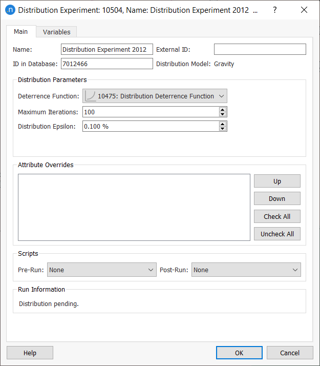
3. Select Distribution Model: Gravity Model and define the experiment parameters as follows:

   
   

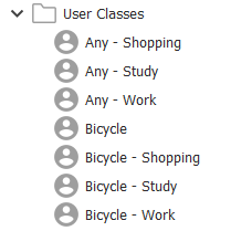
   The distribution step distinguishes by purpose but not by mode, therefore, before running the experiment we must create a user class (vehicle type + trip purpose) considering all vehicle types for each trip purpose (shopping, study, and work). 4. Create a new user class for work and complete its parameters as shown below.

   
   

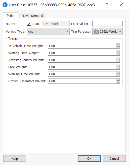
4. Create user classes for shopping and study in the same manner.

   
   

5. In the scenario dialog, on the Outputs to Generate tab, tick Distribution Results: Store.

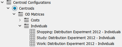
6. Run the experiment. The Outputs tab will display the results on the Summary subtab.

   
   

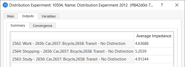
7. From this dialog, we can generate the OD matrices required for Exercise 3. To do so, click Generate Matrices. The matrices are added to the Project window:

   
   

Exercise 3. Running a Modal Split

Data inputs relevant to this exercise

• Centroids
• Distribution and modal split data sets
• Distribution and modal split area types
• Time periods
• Parking area types
• Transportation modes
• Trip purposes
• User class occupancies
• Skim matrices
• Modal split functions

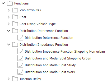
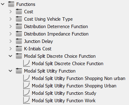
To run a modal split, we need to assign the modal split functions to the distribution area. These functions are pictured below and you can find them in the Project window as usual.

To run a modal split:

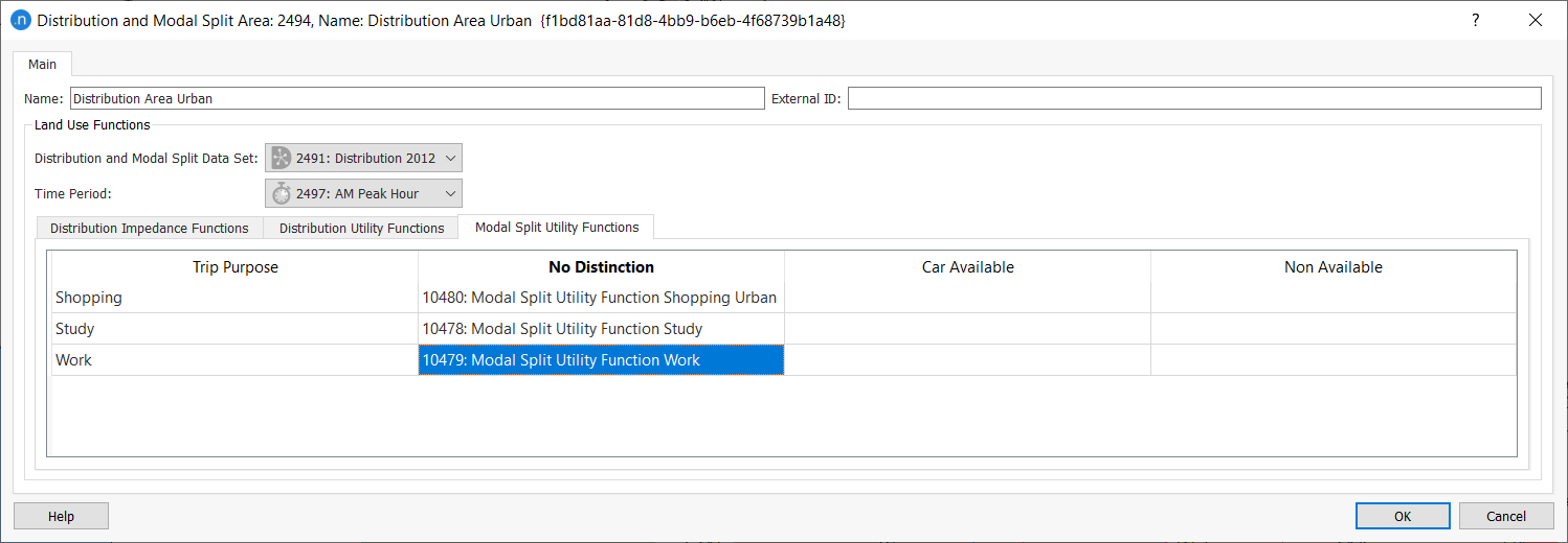
1. Open the distribution area named Distribution Area Urban and click on the Modal Split Utility Functions subtab.

2. Alongside Trip Purpose Shopping, Study, and Work, select the modal split functions as shown below in the No Distinction column.

   
   

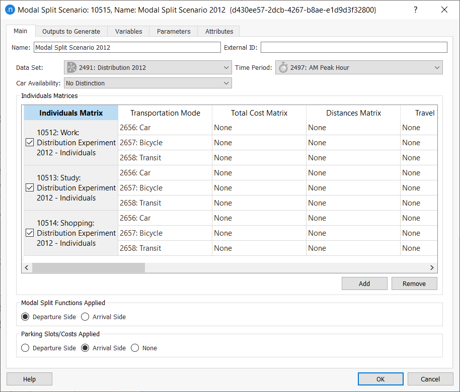
3. Select Scenarios > New > Modal Split Scenario and define the parameters as follows:

   
   

4. Right-click on the scenario and select New Experiment.

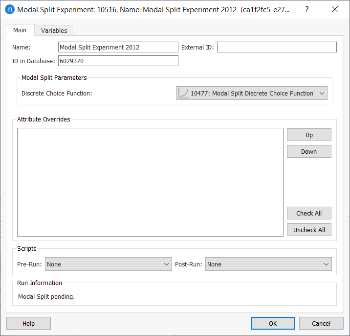
5. Double-click on the experiment and define its parameters as follows:

   
   

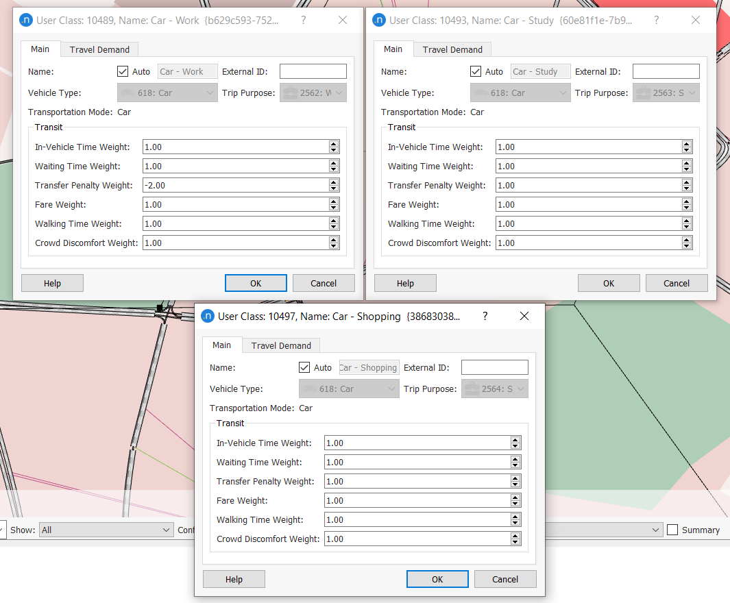
   For transit, we need to know the number of individuals (users of transit: passengers). But the demand matrices for private transport should contain the number of trips (users of the private network: vehicles), not individuals. We will therefore add information to the user classes we are using by providing the vehicle occupancy for user classes with the vehicle type Car, for each purpose. Bicycles don't need to be updated as the default is 1 individual and 1 trip. 6. Create three user classes: for Car – Work, Car – Study, and Car – Shopping and complete their parameters as follows:

   
   

   We will assume that the City Business District (CBD) has a restricted number of parking spaces and we will provide this information for the CBD. 7. Open the CBD area. 8. Add the number of Parking Slots as pictured below.

   
   

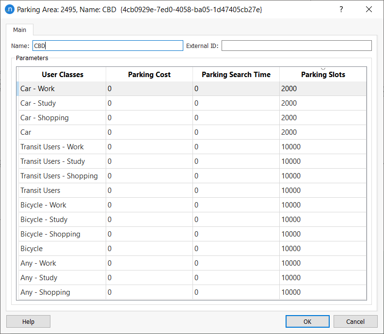
   We have specified 2000 spaces exclusively for cars that go to the CBD for work, plus 2000 for cars that go to the CBD for any purpose (work included). For the rest of users, there is no parking restriction so we set the number of available slots to a number which is high enough. 9. Right-click on the experiment and select Run Modal Split. The Outputs tab will display the results on the Summary subtab (your results might vary).

   
   

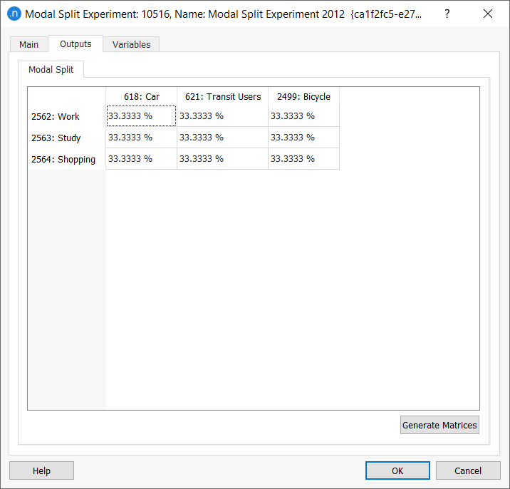
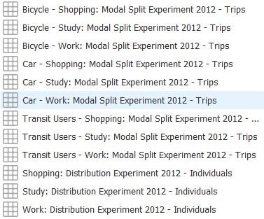
6. Click Generate Matrices to generate the OD matrices for static assignments. They will appear in the Projects window, as pictured below.

   
   

Exercise 4a. Running a Static Assignment

Data inputs relevant to this exercise

• Network
• Cost functions
• Private traffic demand matrices

In this exercise, we will assign the demand into the network. We have obtained nine matrices of demand from the distribution and modal split experiments.

Now we will create three traffic demand objects – one for each mode of transportation (bicycle, car, transit) – and add the three corresponding matrices to each demand. We need to do this because we are going to use a different assignment method for each transportation mode.

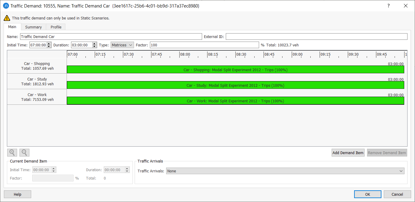
For example, the Traffic Demand Car will contain three OD matrices for the three user classes associated with vehicle type Car.

To add the new traffic demands:

1. In the Project window, Right-click on Traffic Demands > New Traffic Demand.
2. Rename it Traffic Demand Car.
3. Open the new demand and click Add Demand Item.

4. Tick the three car-related demand item and click OK. Your demand should look like this:

   
   

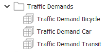
5. Repeat steps 1–4 but for bicycles and transit modes. You should have the following set of demands in the Traffic Demands folder.

   
   

Now we will add scenarios and experiments. Firstly, two static assignments followed by one transit assignment.

To add the two static assignments:

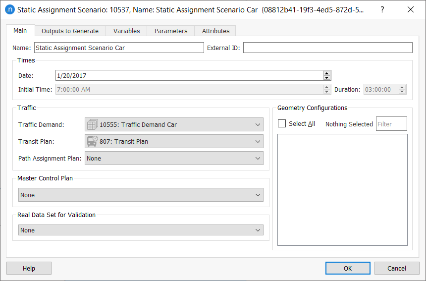
1. Create two static assignment scenarios and one transit assignment scenario.

2. For the first static assignment, select the Car demand and select a Frank & Wolfe (equilibrium) experiment.

   
   

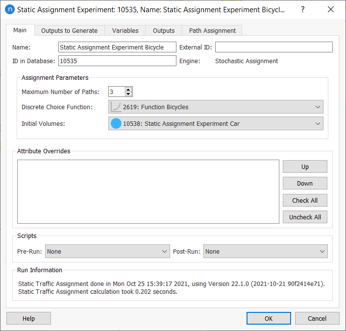
3. For the bicycle static assignment scenario, select a Stochastic Assignment.

4. Set its Maximum Number of Paths to 3.

5. Select Discrete Choice Function as Function Bicycles. 6. Set the pre-loads (Initial Volumes) in the network to use Static Assignment Experiment Car.

   
   

To add the transit assignment:

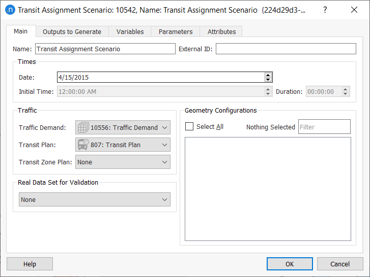
1. Create the transit assignment scenario and complete the parameters as shown below.

   
   

2. Click the Outputs to Generate tab and select the outputs to save: Sections and Transit Stops.

   
   

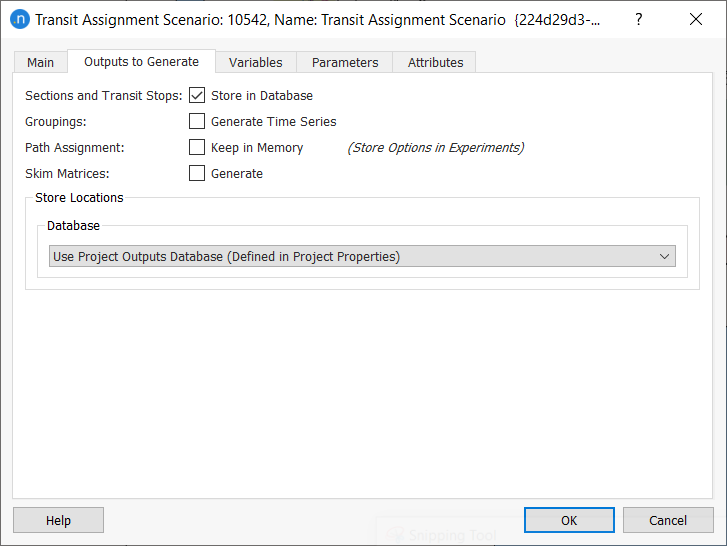
These will be stored in the database, with the ID of the experiment. Select these options for each scenario.

Path assignment results are stored in an APA file. Information about the file is contained in a path assignment object and is specified at the experiment level. So we now need to create three path assignment objects.

A path assignment contains the path where the file is located plus information about which experiment produced the data and which experiments are using them as inputs.

To create a path assignment:

1. Select Demand Data > New Path Assignment.

2. Open the new object to see its parameters.

   
   

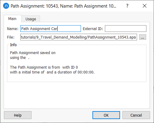
3. Rename it Path Assignment Car.

4. Repeat steps 1–3 for Bicycle and Transit.

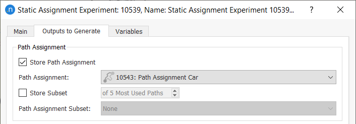
5. To store the path assignment data, open the relevant experiments, go to the Outputs to Generate tab, tick Store Path Assignment and select the correct Path Assignment object from the drop-down list.

   
   

Before running the car-related static assignment experiment, we need to create three function components to retrieve some extra outputs from the assignment. These components will be travel time, distance,and speed.

To add function components:

1. In the Project window, right-click Functions > New > Function Component.

   
   

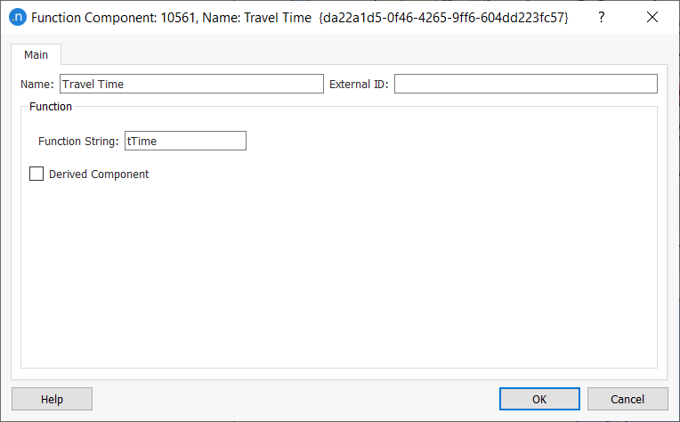
2. Define the travel time component as shown below.

   
   

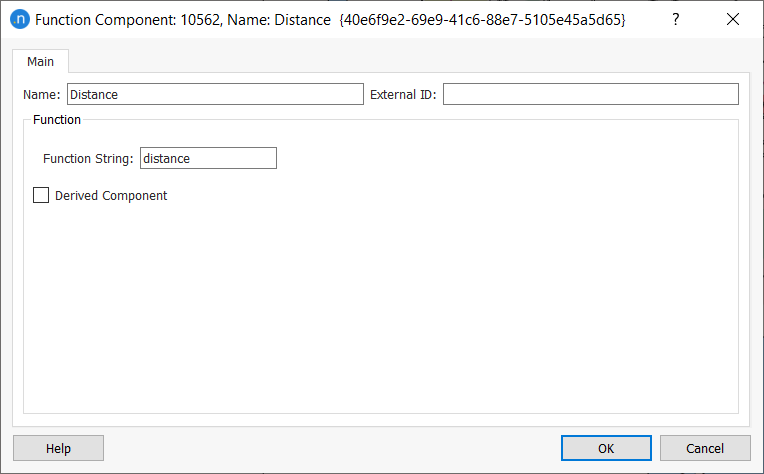
3. Repeat steps 1 and 2 for distance.

   
   

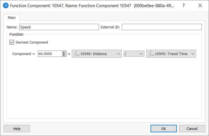
4. Repeat for speed, which is a derived component and requires the following more complex parameters:

   
   

To run the assignments:

1. Run the car-related static assignment first by right-clicking on the experiment and selecting Run Static Traffic Assignment.

   
   

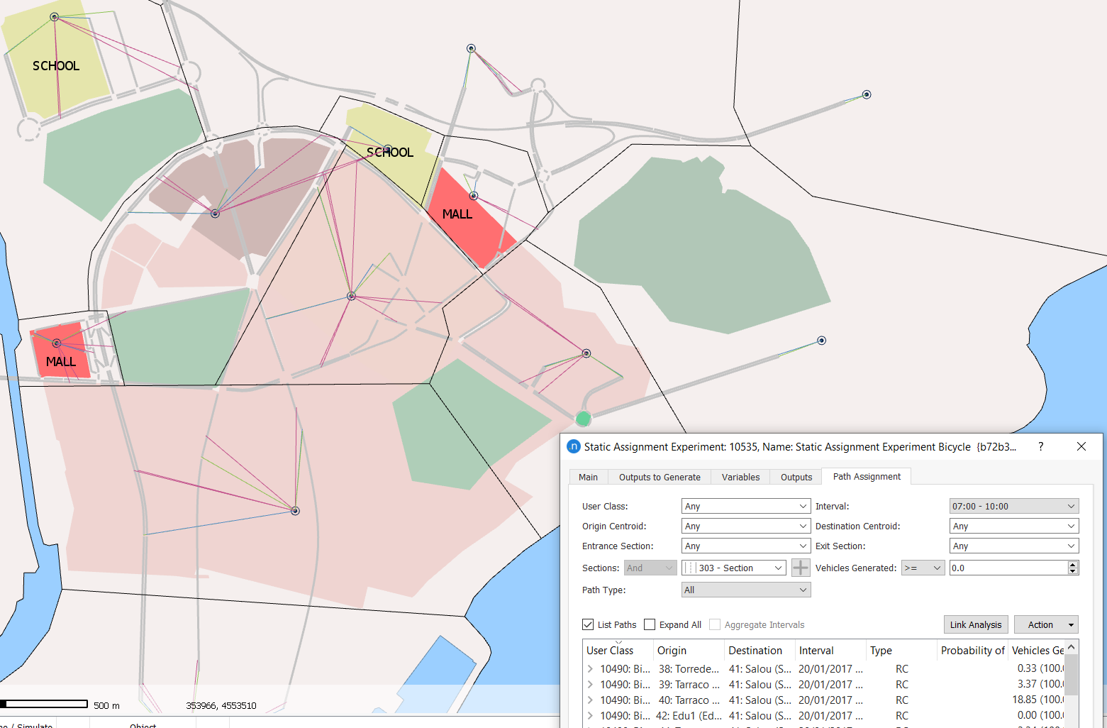
   The path-choice results are displayed on the Path Assignment tab of the static assignment experiment dialog. Take a look at the results and change the values of the parameters to explore the outputs, e.g. select a road section and click Link Analysis to see the paths of vehicles traversing that link.

   
   

2. Now run the bicycle-related static assignment experiment. This assignment takes into account the car assignment results in the initial volume settings, and should be run second.

Exercise 4b. Running a Transit Assignment

Data inputs relevant to this exercise

• Network with centroid connections to and from transit stops
• Walking transfer costs
• Fare system
• Cost functions
• Passenger demand matrices

We have already set up the transit demand (in numbers of passengers) and the transit scenario, but we haven't run the transit assignment yet. First, let's create a transit zoning system and learn about some of the options available in the transit assignment experiment.

To set up the transit assignment experiment:

1. Right-click on the transit scenario and select New Experiment.
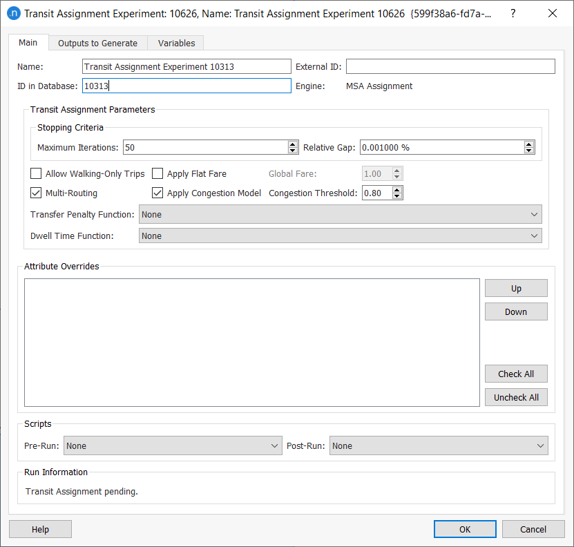
2. For the Assignment Method, select MSA Assignment.

3. Complete the experiment's parameters as pictured below:

   
   

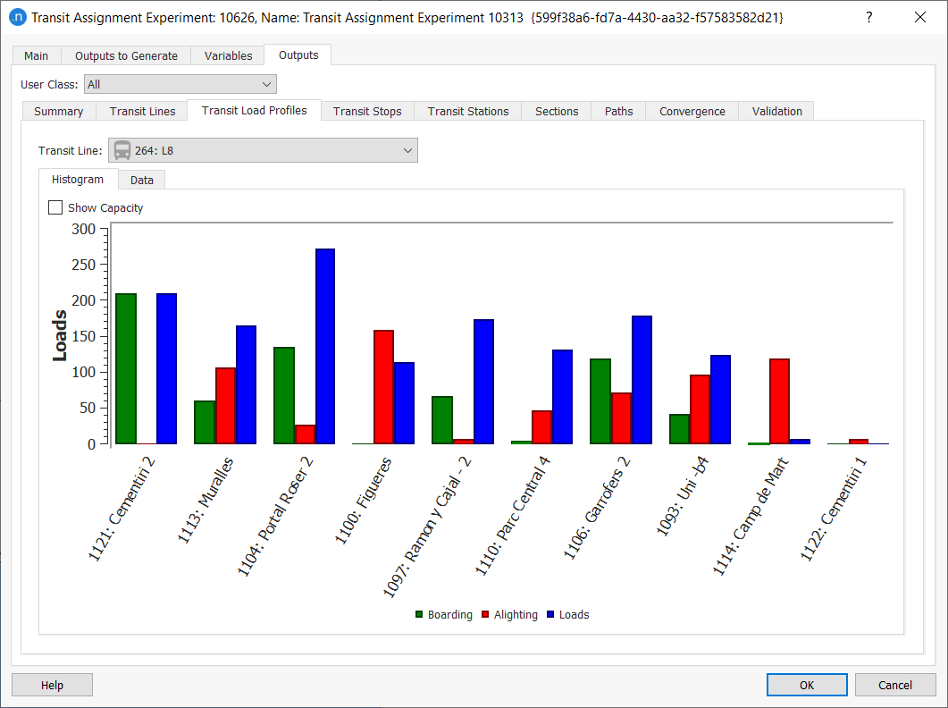
4. Run the experiment. The results are displayed on the Outputs tab and its array of subtabs:

   
   

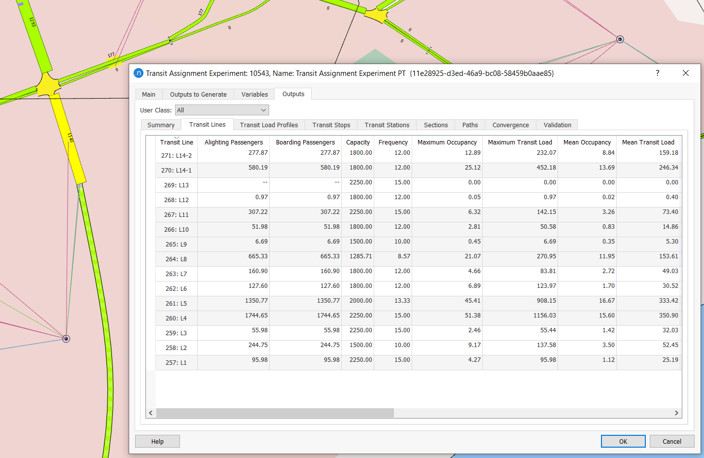
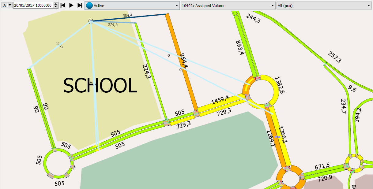
5. Check the assignment loads on the various subtabs.
   

Exercise 5. Running a Four-Step Model Experiment

In this exercise, we will bring the previous processes together by designing a four-step experiment diagram that contains all the steps we have completed so far. Such a diagram is also useful for keeping track of the process that was developed to run the project.

To run a four-step model experiment:

1. Create a new four-step model scenario and add an experiment to it.

2. Open the experiment. You should see a blank grid as pictured below.

   
   

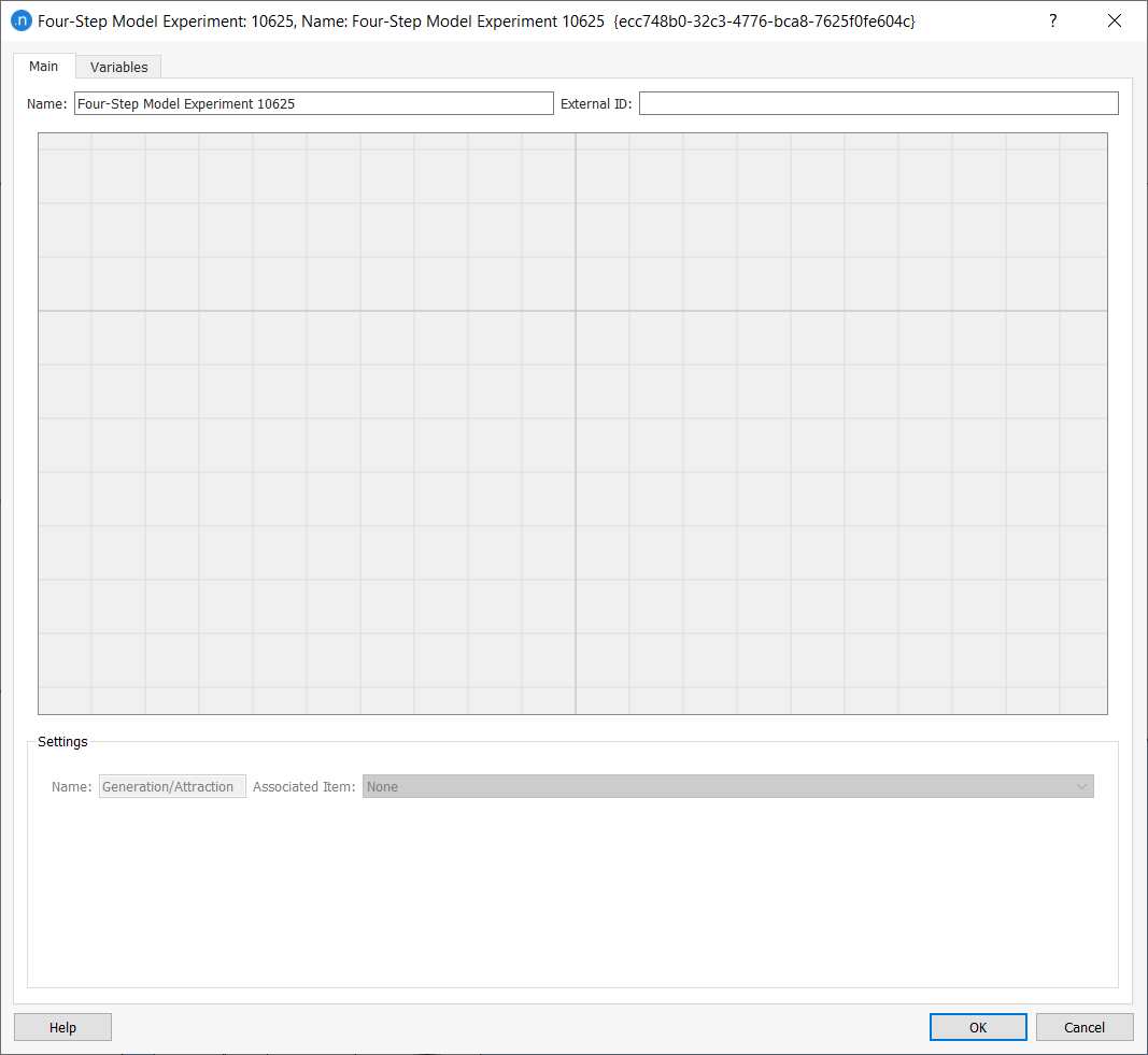
   In this space we can define the four-step model diagram, which consists of interconnected boxes that represent the experiments and outputs we have generated so far in this tutorial.

3. To add boxes, right-click on the grid and select the appropriate category (e.g. Generation/Attraction, Distribution, Modal Split, Skim Matrix, etc.).

   
   

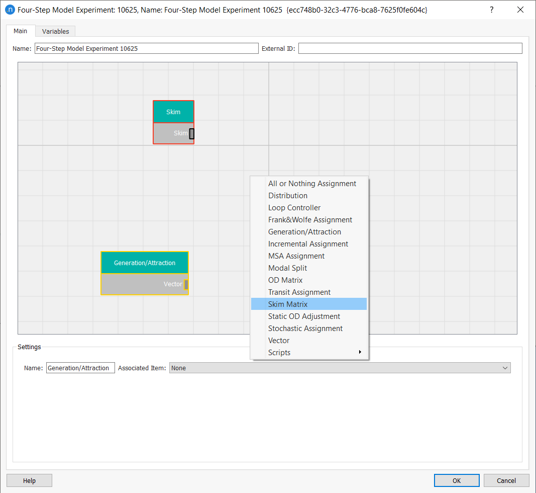
4. Add all the boxes related to the processes we have run so far and link the boxes together by dragging links with the mouse from one box to another. Aim to produce the result pictured below.

   
   

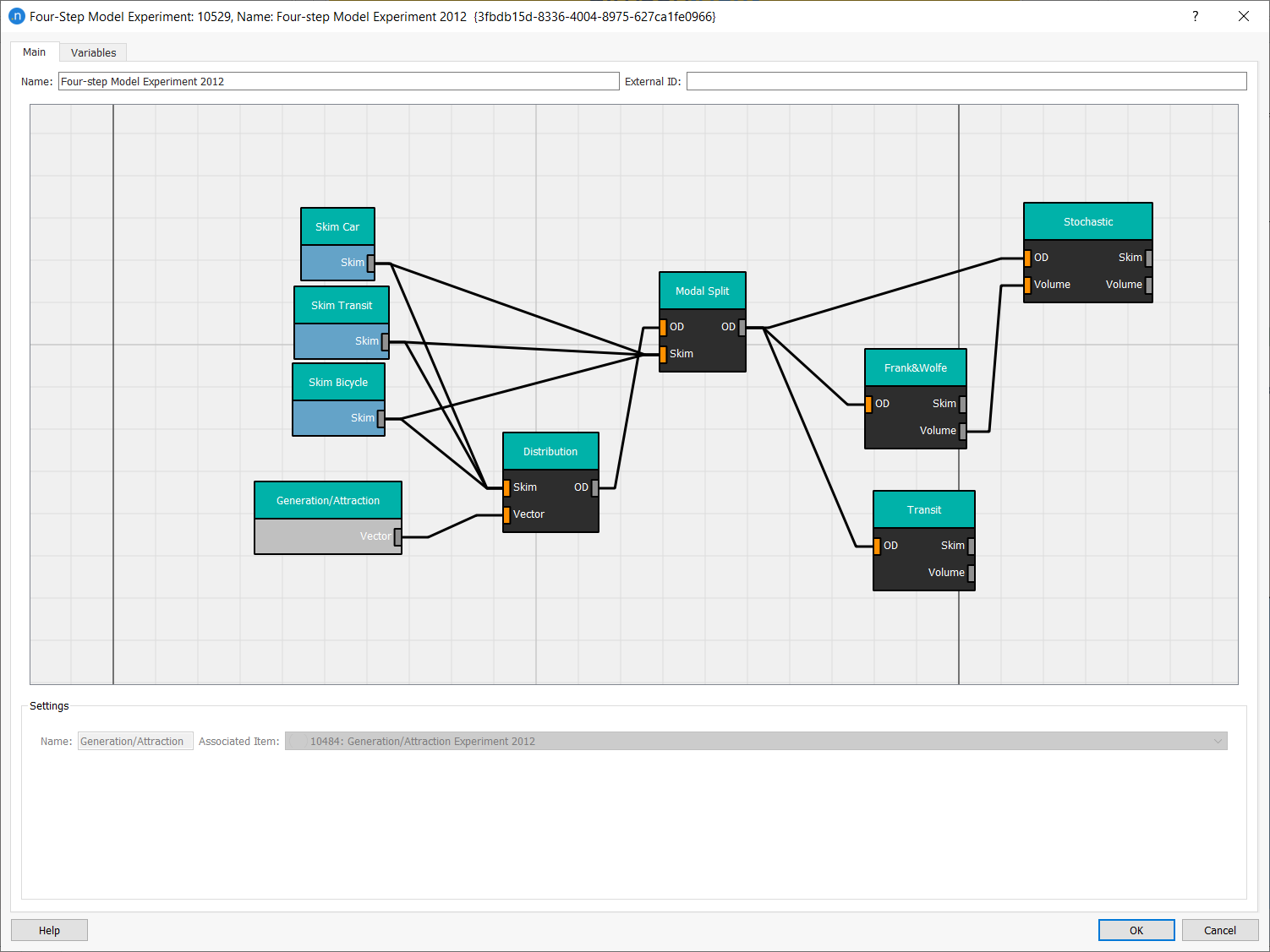
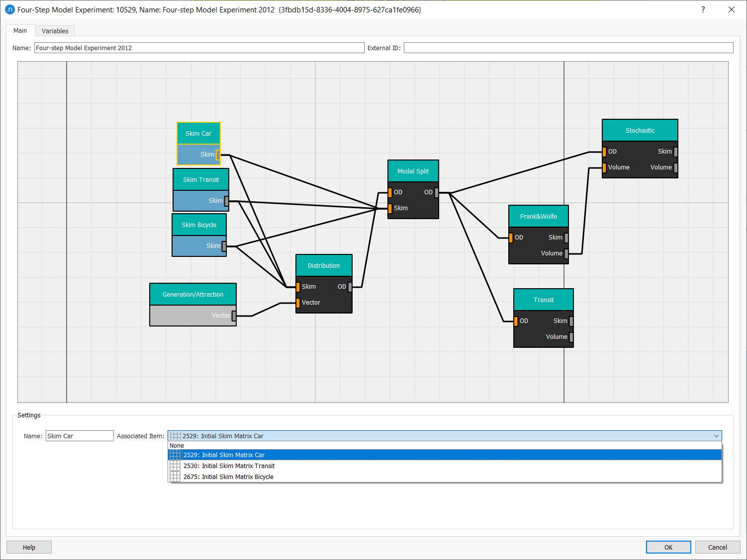
5. Complete the Settings information for each box and arrow. The first screenshot below shows how to link the Skim Car box with its Associated Item from the drop-down list.

   
   

   The next screenshot shows how to link the Modal Split process box to the correct modal split experiment.

   
   

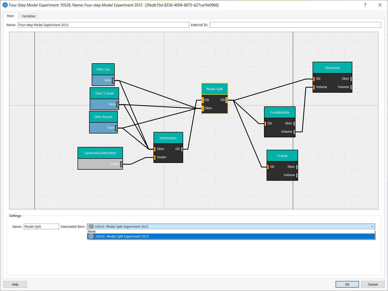
   Make sure all the boxes and links are associated with the correct outputs and experiments.

   
   

6. Run the experiment from the Project window by right-clicking on it and selecting Run Four-Step Model.

You can further define the boxes in the diagram and reuse output skims from assignments for a second distribution, looping on the second-third-fourth steps.