Map-Based Outputs

Map-based outputs are shown in the View Windows and can display map-based data from the road sections, junctions or centroids, or they can display animated data in 2D or 3D showing the movement of vehicle and pedestrians in the simulation.

Information shown in the map view is not necessarily limited to simulation outputs, static information can also be displayed and used to debug networks and identify coding anomalies.

Map Window

The data shown in the 2D view is controlled by the View Mode dropdown menu which selects one of View Modes available in the project. View Modes are created and edited using the View Modes Editor and select what data is shown in the map view. How this data is then presented on the map is controlled by View Styles which are created and edited by the View Styles Editor.

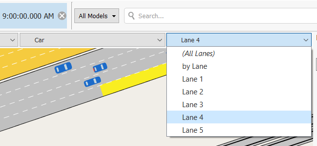
Any further details required are also selected in the "View Mode" drop down boxes, such as an option to disaggregate flows by vehicle type and by lane. The figure below shows Car and Lane 4 selected, but All is available for both.

The Data Source dropdown menu controls the source of the data. This can be a static experiment, a dynamic experiment average or a dynamic replication. The source "Active" uses the currently selected experiment.

View Navigation

Moving around the map view with the standard navigation tools is documented in the View Navigation Section of the GUI Manual

Time Toolbar

The Time Toolbar controls the time and date in the simulation used to retrieve the data from the Data Source. If the source is a dynamic simulation, the Play button will start an animation displaying the results as specified in the view mode at the time interval specified in the Scenario Editor: Output Tab. The resulting animation will show how the road network conditions vary with time i.e. how congestion rises and falls over the peak period.

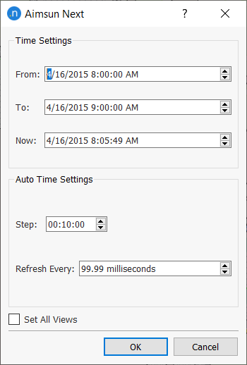
The Set Time dialog is displayed from the View menu of the main window. It controls the time displayed in the view; the now setting moving the display to the chosen time. It is also used to change the range, speed, and data interval of the animated data display. In the example below, the data is displayed between 08:00 - 09:00 at 1 minute intervals with the animated data display updated every 50 milliseconds resulting in a 3 second display, started by the Play button in the time toolbar.

View Modes

A View Mode is a combination of several View Styles that are applied at the same time. A view mode is then applied to a 2D view to modify how the network objects are displayed using static or dynamic information.

A View Mode will often have several view styles attached to it which change the display of objects to assist the user in interpreting the behavior in the model. Styles can be applied at different levels of zoom, for example a view mode can display a section related measure by lane at close zoom levels but as a section aggregate at higher zoom levels. Styles can be complementary, using different objects displaying for example lost vehicles and nodes where vehicles get lost. Styles can use dynamic data where the display will be updated as the simulation runs to display network behavior or they can be static and used to find network coding anomalies, for example displaying section types in different colors to assist the user in spotting any discontinuity in road type.

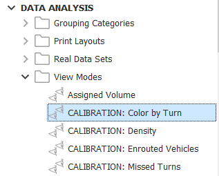
The view modes are listed in the Project Window in the Data Analysis folder.

Creating a new View Mode

Select the New / Data Analysis / View Mode option either in the Project Menu, in the Project Window Data Analysis folder context menu or in the Project Window View Modes folder context menu. Alternately, create a new View Mode using the Wizard Dialog which is accessible via the Tools menu, Data Analysis sub menu.

View Mode Editor

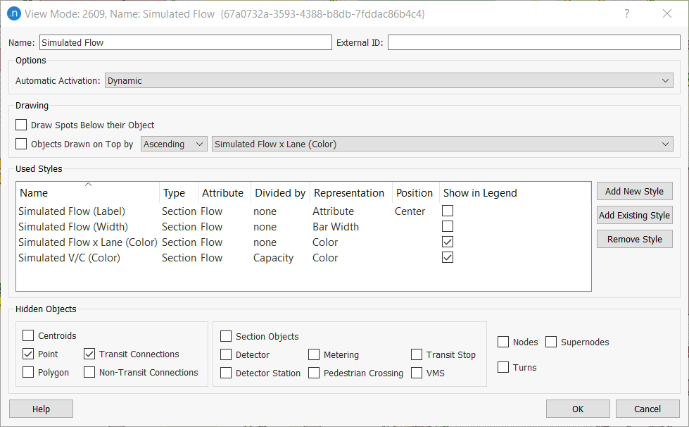
The View Mode editor is used to assign view styles to the mode. The dialog contains a list of any view styles that are assigned to it. It also enables you to hide certain objects without using a view style to do so.

The view mode automatic activation options are:

• Never: The mode will never be activated automatically.
• Micro: The mode will be activated when a Microscopic simulation finishes.
• Meso: The mode will be activated when a Mesoscopic simulation finishes.
• Macro: The mode will be activated when a Macroscopic Traffic assignment finishes.
• Hybrid: The mode will be activated when a Hybrid simulation finishes.
• Dynamic: The mode will be activated when a dynamic simulation is running.
• Paths: The mode will be activated when checking the paths from any dialog (i.e. Replication editor: Path Assignment tab folder).

The Drawing options are:

• When drawing styles using spots, these spots are drawn: either after drawing all the objects in the layer (in this case the spots will be over the objects) or before drawing the objects (in this case the sport will be behind the objects). If the style uses big spots is a good idea to draw them behind the objects to clarify the plot.
• To set the drawing order of objects in a layer (each layer will be drawn in the order specified by its level) based on the value of the attribute used in one of the styles in the mode. The sorting will occur only when selecting the view mode. Combined with the previous option can help to clarify a view mode (for example when drawing isochrones).

The View Styles box contains a list of the View Styles attached to this View Mode. Options are available to add or remove existing view styles or to create a new one.

Hidden Objects

A common use of view styles is to hide objects of a certain type (e.g. all centroids) to add clarity to the view by removing clutter. However, the Hidden Objects options on the View Mode editor enable you to hide common types of objects in the view mode without needing to create a specific view style to hide them.

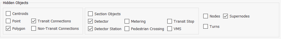
To hide objects:

1. To hide all centroids, tick Centroids.
2. To hide some aspects of centroids, untick Centroids and select one or all of the following:
3. Point (hide centroids' points)
4. Polygon (hide centroids' zonal polygons)
5. Transit Connections (hide connections between centroids and transit stops)
6. Non-Transit Connections (hide connections to between centroids and road sections)
7. To hide all sections, tick Section Objects.
8. To hide some objects in sections, untick Section Objects and select one or all of the following:
9. Detector
10. Detector Station
11. Metering
12. Pedestrian Crossing
13. Transit Stop
14. VMS
15. Tick Nodes, Supernodes or Turns to hide these objects.

Some of these object-visibility options are also available for quick access from the Legend Window.

View Mode Examples

Vehicle Marked by Origin

The following example will create a View Mode that colors the vehicles according to their origin centroids.

Create a New View Mode and call it Vehicles by Origin. Create a new Style and add it to the new mode. Edit the new style.

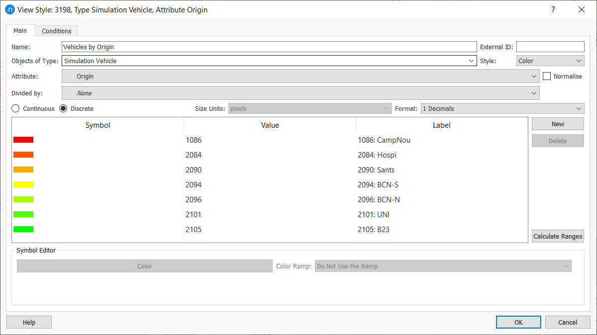
In the style editor, shown in the previous figure, choose Simulation Vehicle as the Type and Origin as the Attribute. Change the type of the variable to Discrete. Keep Color as the Representation.

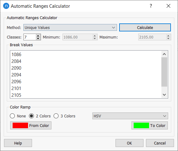
Press the Calculate Ranges button. In the Automatic Ranges Calculator dialog (next figure), choose Unique Values as the Method. Press Calculate to get all the unique values. Press OK.

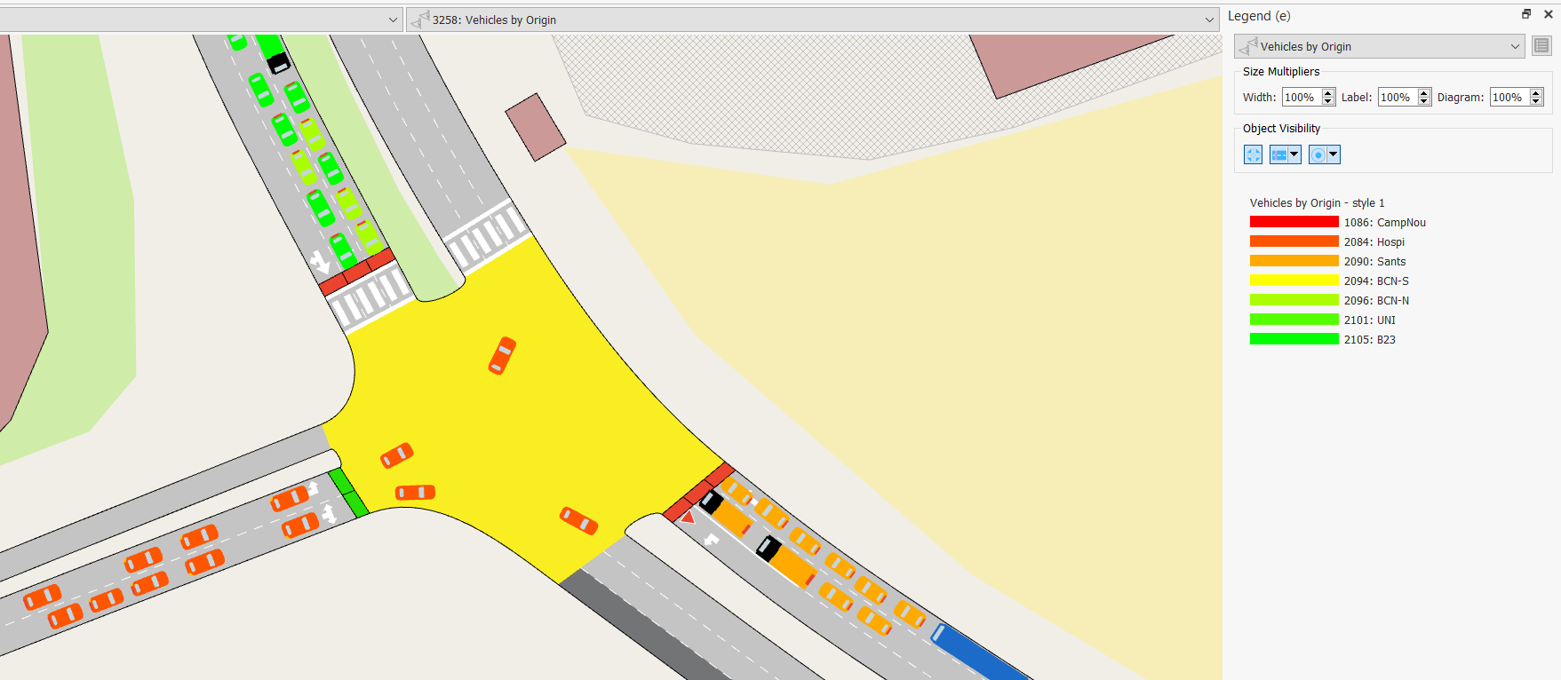
Edit the ranges if necessary. Select the new mode from the Drawing Mode list in the current view.

Hide Centroids

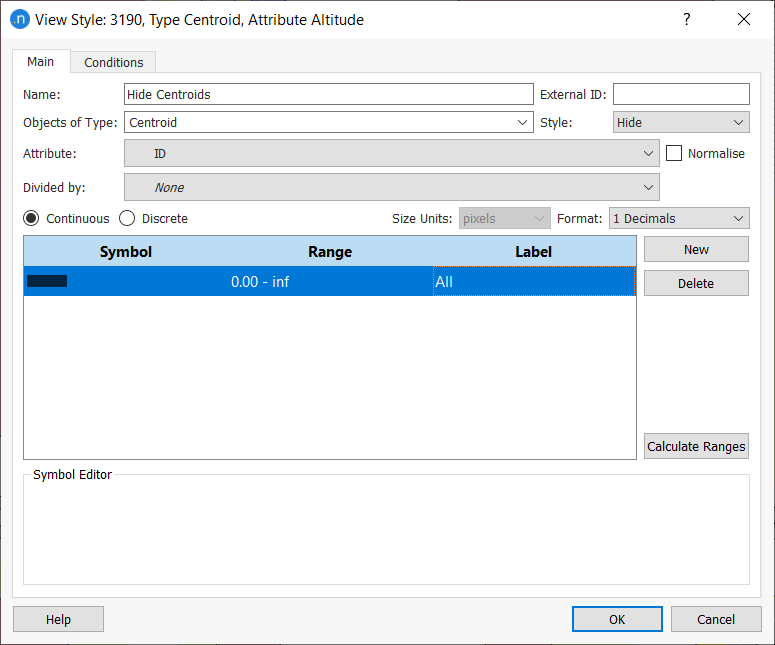
Next example will create a View Mode where centroids are hidden. Create a new mode and call it Hide Centroids. Create a new style and add it to the new mode. Edit the new style.

In the style editor, shown in figure below, choose Type: Centroid and Attribute: ID. Set the type of the variable to Continuous and the Representation to Hide. Press the New button and set the range to 0.00 – inf.

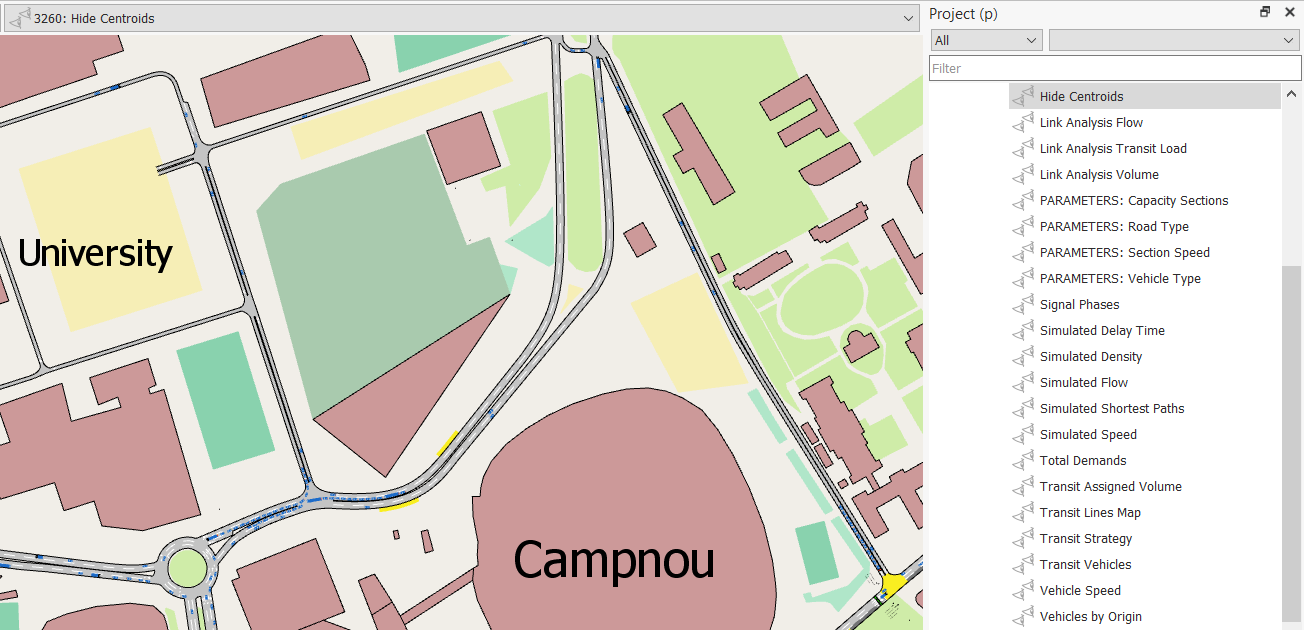
The next figure shows the network with the View Mode set to Hide Centroids.

View Mode Wizard

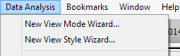
The View Mode Wizard is started from the Data Analysis Menu.

This wizard will assist the user in the creation of a new mode and optionally assigning some existing styles to it. The figure below shows the wizard dialog, which is used to define the mode name as well as to decide whether to use existing styles, create a new style or adapt an existing one.

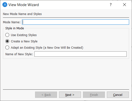
When selecting Use Existing Styles a list of styles will be shown. If the user chooses to Create a New Style then the steps followed in the View Style Wizard section must be done and finally, if the option chosen is to Adapt an Existing Style, then a window to choose the existing style to adapt and the style attribute will be shown.

Default View Modes

The default View Modes supplied in the standard Aimsun templates are:

• Calibration: Color by Turn: This view colors vehicles by the next turn they plan to make. It is useful in the calibration stage of a model to see how vehicles use lanes as they approach the next junction.
• Calibration: Vehicles with En-Route Path Update: This view marks those vehicles which have updated their path en route in red, allowing them to be easily seen in the simulation.
• Calibration: Missed Turns: This view has five associated view styles which mark nodes where vehicles have missed turns with a color which denotes how many have been missed and with a label to quantify that number. It also marks vehicles which are lost by color, those which have no route to their destination or that have missed turns, and those with a label to indicate their first missed turn. Once again, this is useful in the calibration and model debugging stages.
• Calibration: Virtual Queue SI: This view marks those sections with a virtual queue with a color and with a label to show the size of of the queue. As with all default views, prefixed "Calibration: it is intended to assist in calibrating the model.
• Generals: Graph: This view reduces the detail in the map and shows cars and transit vehicles as larger different colored circles, providing a more visible view of car and transit interactions.
• Parameters: Capacity Sections: This view reduces the detail in the map and colors sections by capacity. The view is useful in model building as any disparity in capacity will be made obvious.
• Parameters: Road Type: A similar view which colors sections by road type and is intended to assist the user in finding modeling errors in specifying road type.
• Parameters: Sections Speed: A similar view which colors sections by speed limit and which is intended to assist the user in finding modeling errors in specifying speed.
• Parameters: Vehicle Type: This view colors vehicles by type, overriding the vehicle's modeled color while the view is active. It is intended to assist in model calibration and debugging.
• Simulated Delay Time: This view shows the delay time simulation output for the section as a legend and as a colored width where a wider line shows more delay. As the view zooms in closer, the delay is shown by lane color rather than by line width.
• Simulated Density: This view shows the density simulation output for each section as a legend and as a colored width where a wider line shows higher density. As the view zooms in closer, the density is shown by lane color rather than by line width.
• Simulated Flow:This view shows the section flow simulation output divided by the section capacity as a legend and as a colored width. This shows where capacity is close to the limits. At close levels of zoom, it shows the flow by lane color.
• Simulated Speed:This view shows the speed simulation output for the section as a legend and as a colored width where a wider line shows more delay. At close levels of zoom, it shows the speed by lane color.

Once the simulation is finished, a new automatic view mode is created:

• Simulated Shortest Path: This view hides the normal section and node display and re-displays the sections using the "mark" variable. If the experiment or replication "Path Assignment" properties dialog tab is opened and a path selected, it will be "marked" and shown in this view. Note that this view assumes an interaction between the view and another dialog; this view mode technique can be used in other views where the status of a section or node can be changed and the view used to observe where changes occur.

This list of View Modes is not exhaustive. As experiments of different types are run, appropriate View Modes are added to the list and users can add their own preferred modes as required.

View Styles

A View Style is a means of displaying an attribute of an object. View styles are components of view modes where a mode contains one or more styles which together display information in a 2D view.

Aimsun Next can display any graphical object in a form based on the values of its attributes. It can also show these attributes as labels on the network. For example, it can show sections with a speed of 50 Km/h in red, 60 Km/h in blue, it can draw bars of 3 meters' width on sections with a density of 1,000 and bars of 6 meters' width on those with a density of 2000. These effects are achieved using View Styles.

The view styles are listed in the Project Window in the Data Analysis folder.

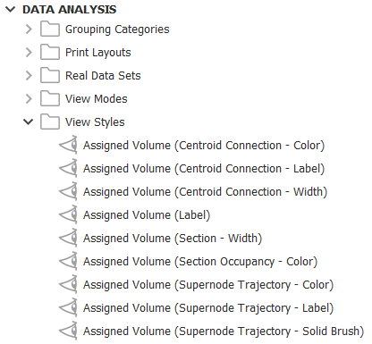
Creating a new View Style

To create a new View Style, select the New…/ Data analysis / View Style option in the Project Menu, or in the Project Window Data Analysisfolder context menu or in the Project Window View Styles folder context menu. Once created, the new View Style will appear in the View Styles folder inside the Data Analysis main folder in the Project Window.

It is also possible to create a new View Style using a Wizard Dialog accessible via the Tools menu, Data Analysis sub menu.

View Style Editor

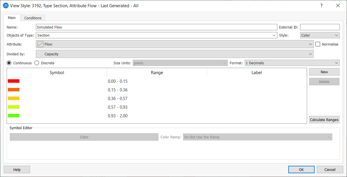
A View Style contains information on:

• The type of object to be drawn (sections, nodes, centroids, polygons…)
• The value of a selected attribute it will be based on (speed, capacity, mean queue, length…). The value can be that of an attribute or the value of an attribute divided by other attribute. Also the values can be normalized if the Normalize box is checked resulting in values ranging from 0.0 to 1.0.
• The style chosen to draw the object (e.g. in red color, using a width of 3 meters, etc.)
• The conditions on when to apply this style, either for a predefined zoom range or based on the value of an attribute.

The following table shows the different ways the object can be drawn:

Type Effect

---

Color Changes the color Bar Width Changes the bar width Pen Style Changes the pen style Brush Style Changes the brush style Spot Draws a spot (circle, start...) over the object Hide Hides the object Color Opacity Changes the opacity of the colors defined in another style Attribute Adds a label with the value of the specified attribute Diagram Draws a diagram (circles, pies, histograms...) on each object Stacked Bands Available for sections. Width as a set of multiple bands

After selecting the object, the attribute, and the style used to draw it; different values for the attribute are specified which will affect the drawing style. For example, the pen used to draw a section be changed in width by speed band or the spot used to draw a vehicle can both colored by acceleration rate.When a label is displayed, the number of decimal digits to use in the label can also be specified and when defining a style that displays a label or a spot, the size units can be defined in meters or pixels.

An attribute can be either continuous or discrete. Continuous attributes are assigned a drawing effect by range, discrete attributes are assigned a drawing effect by value. The Calculate Ranges Button can be used to calculate automatic ranges.

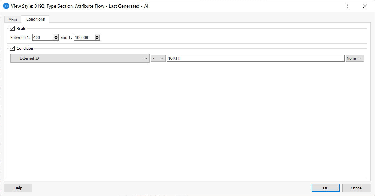
In the Conditions tab (see next figure), the zoom range (meters elevation) for this style can be specified. The zoom range can be used to change the level of detail shown in the view, for example a section can have lanes colored by flow rate when lanes are clearly visible in the view but as the view zooms out, the style switches to show the average flow for the section.

The conditions tab also specifies if the style is to be applied to a subset of objects. This subset can be specified by selecting the attribute of the object to filter by and the range of matching values to apply the view style. Multiple conditions can be used ( i.e. Vehicle is Transit and capacity > 30).

View Style Wizard

The View Style Wizard is started from the Data Analysis Menu.

This wizard will assist in creating a new style and optionally assign it to an existing view mode. The example here shows how to create a style that will color the sections based on the section speed.

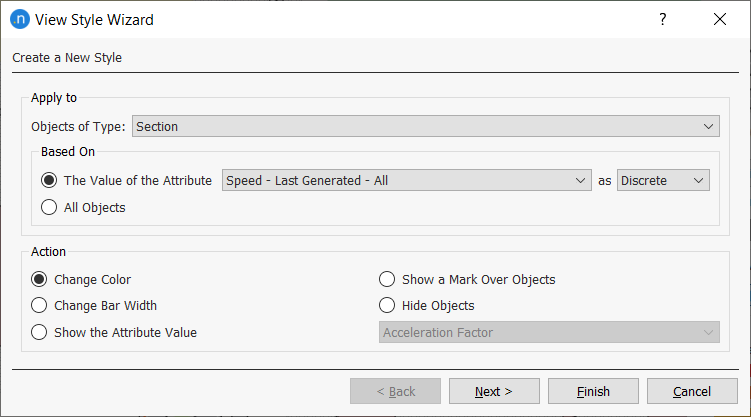
When the Finish button is selected the style will be created with a default group of ranges. If the Next button is pressed, the ranges calculated will be shown and can subsequently be edited.

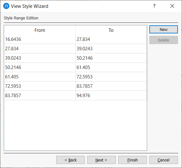
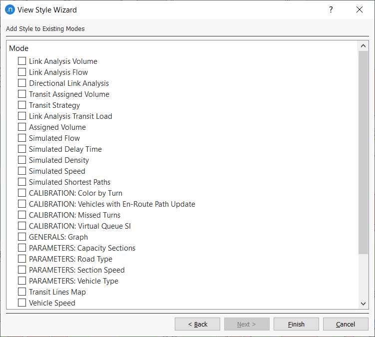
If the Next button is pressed, a list of all the existing modes will be shown . Tick those to which the new style will be assigned.

Automatic Ranges Calculator

There are different methods to classify a set of values:

• Unique values: Creates a class or range for each one of the values.
• k-means: Uses the k-means method to group the different values.
• Quantile: Assigns the same number of values at each class.
• Equal interval(automatic): Uses an automatic interval calculated using (maximum of values)-(minimum of values)/num classes.
• Equal interval(custom): Uses a custom interval calculated using the predefined max and min values.

Select the classification method and click on the calculate button. The ranges are shown in the ranges window.

Dynamic Labels

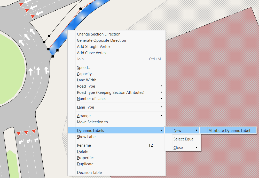
Dynamic labels provides a method of displaying both static and dynamic information about network elements as textual labels. To add a dynamic label to an element, right click on the element in the 2D view to access its context menu, then select Dynamic Labels /Attribute Dynamic Label.

Select the required label, in this case, the detector name,

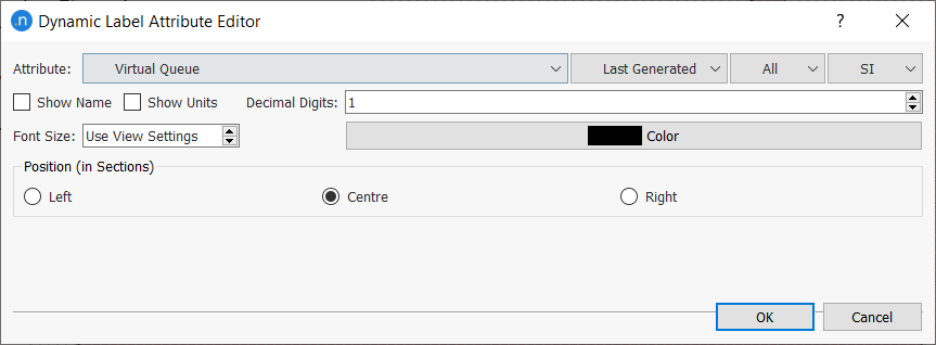
Check tick boxes to show attribute name, units, change the color or the font size if required, then select OK in the editor. The label will appear over the element, but it can be dragged to any position.

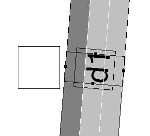
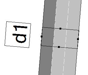
Multiple labels can be added, in this case the SI Section Speed as well as the name.

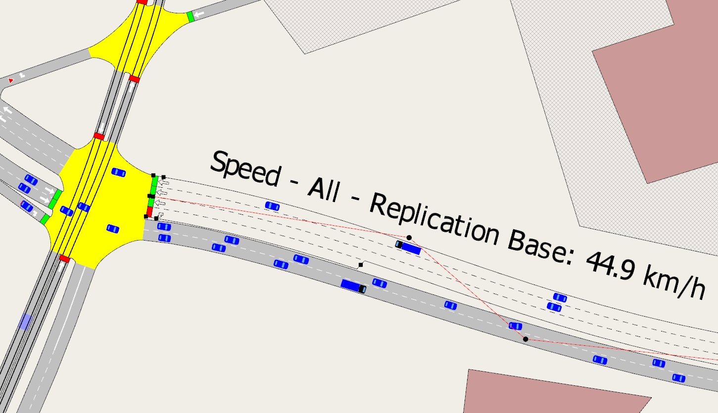
Being dynamic, labels are updated with relevant information, for example during a running simulation at the data update period.

Labels can be added to more than one element at once by selecting all (for example by holding down the [Shift] key) then selecting from the context menu on a selected element as normal.

Dynamic labels can be closed by selecting the label or labels, and either pressing the [Delete] key, or by selecting Dynamic Labels / Close / Selected from a label’s context menu. Selecting Dynamic labels / Close / All closes all labels in the view, while Dynamic Labels / Close / Equal closes all labels in the model of the same type as the first label selected.

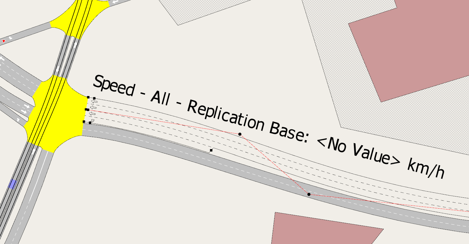
Analyzer Dynamic Labels are specific to turns. Right click the node to be analyzed and select Dynamic Labels / New / Analyzer Dynamic Label (see next figure)

The Node Analyzer Editor Dialog is used to select any Turn Attribute (including time series) and configuring the additional elements to show in the label. After pressing the Ok button, every entrance section in node will have a nearside label showing the information about turns, sorted according the Rule Road Preferences value. The next figure shows an example of Analyzer Dynamic Label.

As normal Dynamic Labels, it is possible to change the label settings by double clicking on any of them.

Legend Window

The Legend window is used to display information about objects shown in a view mode. It can also modify how a view is displayed and how it is annotated, without requiring a new view style.

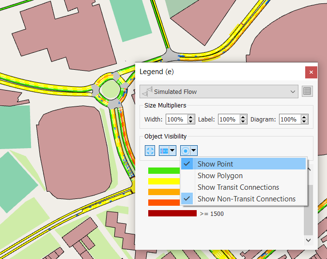
Styles which are selected for display in the Legend window have their range information reproduced in the window to aid interpretation of the display. Within the Legend Window there are options to:

• Change the view mode in use.
• Edit the view mode in use
• Adjust the size of the line width, text size, or circle and square size used to display the attribute in the View Style.
• Toggle the Object Visibility of Nodes, Section Objects (Transit Stops, Metering, Detector, Detector Stations, Parking Space Group, VMS, Pedestrian Crossing), and Centroids (Point, Polygon, Transit Connections, Non-Transit Connections) to quickly show and hide some objects without creating a view style.