Dynamic Scenarios

Dynamic Scenarios are run using micro, meso, or hybrid vehicle-based simulations. They can be run with paths generated externally by the modeler, by another scenario (Static or DUE) or they can use paths based on experienced costs in the network as the simulation runs.

The minimum requirement for a Dynamic Scenario is a base transport network and a Traffic Demand. There are options for a Path Assignment, a Transit Plan, a Master Control Plan and set of Geometry Configurations to be included in the scenario and the Data Output options, Traffic Management Actions, and Real Data Sets can also be specified for the scenario.

Dynamic experiments, in mesoscopic, microscopic, and in hybrid simulations, can also be run using multiple threads on the host computer to speed up execution.

Dynamic Scenario Editor

The scenario editor is divided into several tabs which describe what is to be simulated, the outputs to be collected, the Aimsun Next API and Enhanced APIs in use and the variables they can access, the strategies to be applied to the experiments in this scenario, and parameters to describe the scenario.

Main Tab

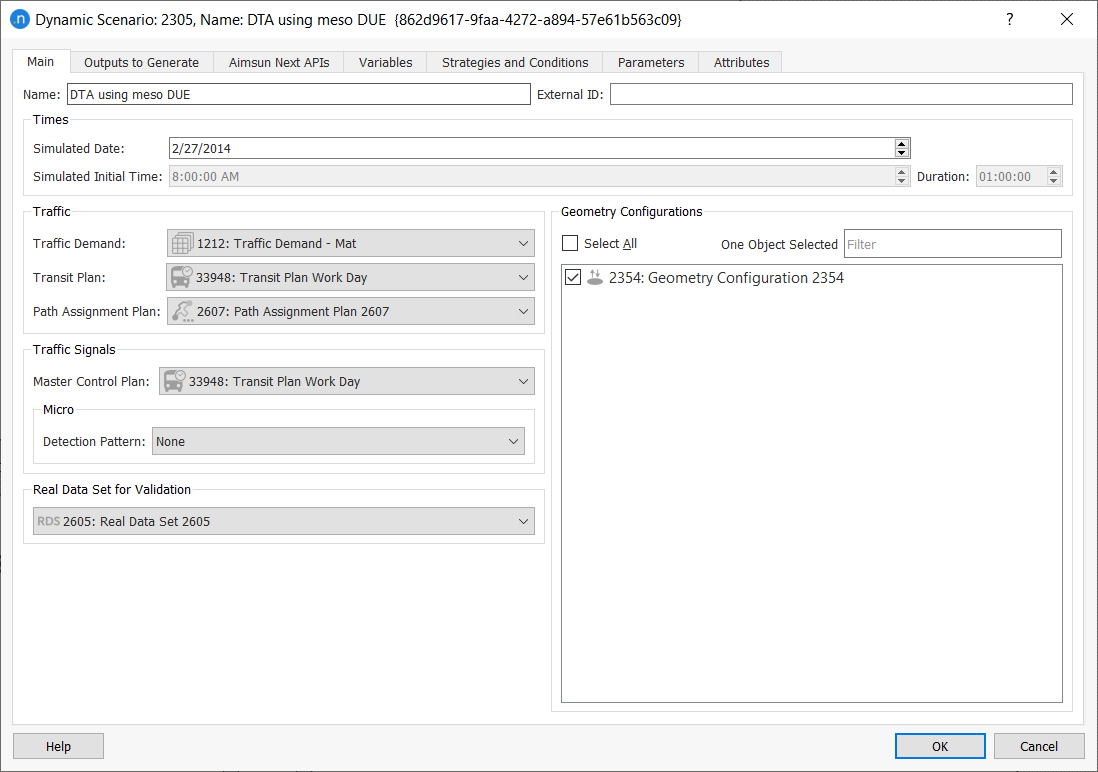
The parameters of the scenario, which will be the defaults for the experiments in this scenario are:

• The name and external ID of the scenario:
• The simulation time and duration: Note the date is for information and not used by the simulation.
• The Traffic information which consists of:
• A Traffic Demand with either OD matrices or a set of Traffic States. This must already exist in the Aimsun document for the entire model, or if this scenario is contained within a subnet, the demand plan must also be contained in the subnet folder for the project.
• A Transit Plan with a set of transit routes and schedules.
• A Path Assignment Plan with a set of routes derived from prior experiments.
• A Master Control Plan which sets the signal control systems for the scenario.
• A Detection Pattern. This is a recording of the vehicle detections made by roadside detectors from a prior simulation. It's prime role is to test adaptive control plans by bringing in the detection data without necessarily requiring the traffic demand that produced the data. Note that if a Detection Pattern is to be created from a Detection Template and a running simulation, then it must be specified in the Scenario which owns that simulation.
• A Validation Data Set: This is data used to compare simulation outputs with observed data.
• A set of Geometry Configurations: These are the variations in the network applied to this scenario.

Outputs to Generate Tab

The Outputs to Generate Tab in the scenario dialog details which outputs are generated by the experiments in the scenario.

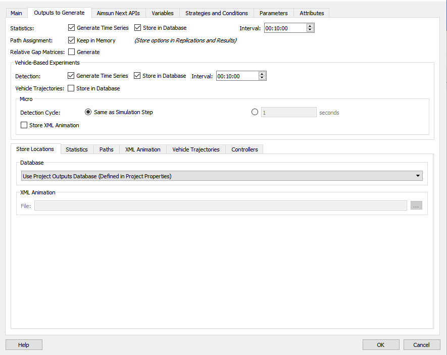
It has the following subtabs:

• Store Locations: Where to store output data.
• Statistics: What data to collect.
• Paths: The path statistics to collect.
• XML Animation: Storing vehicle positions in an XML format suitable for input to Legion.
• Individual Vehicles: The vehicle trajectories are recorded in the database.
• Controllers: Creating Log files for signal controllers.

The details of these output options are documented in the Dynamic Scenario Outputs section.

API Tab

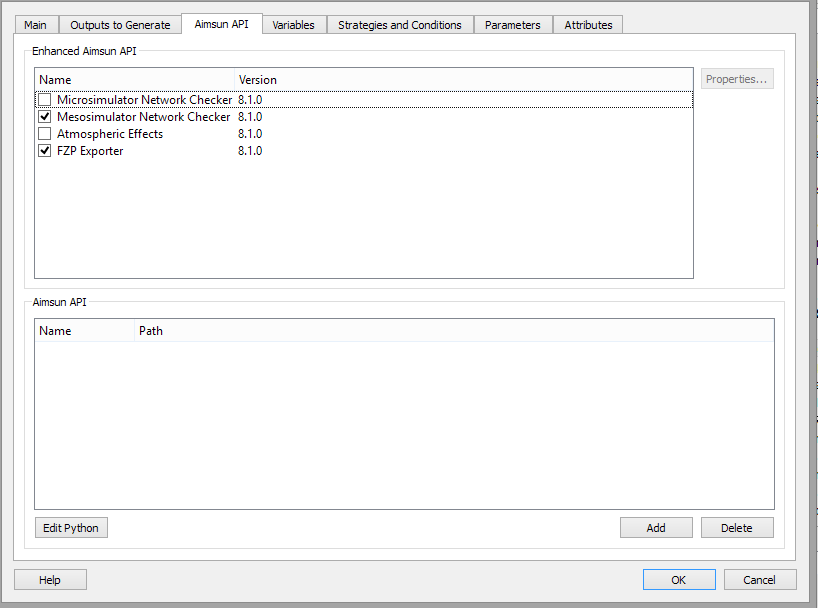
An Aimsun Next API is an external library that the user can create to access the simulator information online during simulation and modify it or check it as needed. The Enhanced Aimsun Next APIs can also access the simulator information and furthermore it gives access to the graphical user interface allowing the creation of new menus, editors, etc. Refer to the Aimsun Next API Manual Section for more details.

In this folder, the available Enhanced API modules are also listed and can be selected to be used in the simulation. The properties button will bring up an API specific dialog where parameters for that module can be defined for the selected module.

Note that to be able to load Aimsun Next APIs an Aimsun Next API license is required.

Variables Tab

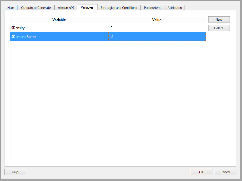
The variables that will be used when simulating any replication from this scenario can be defined in this folder. Note that these variables can also be defined at the experiment level and in that case, the value will be taken from the experiment. When a simulation starts, the variables are assigned their values by looking first at the experiment and, if no value is defined at that level, then at the scenario.

A variable is an arbitrary string that starts with the dollar sign ($speed and$demand are examples of valid variables).Variables can be used in traffic demand items, in policies, in triggers, etc.

For example, a traffic demand defines the factor of a specific OD matrix as $DemandFactor. This demand is assigned to a scenario that contains two experiments. When a replication is selected to be simulated, the simulator assigns the variables to their final values. It looks first in the experiment that contains the replication. If the variable is found there the simulator then uses this value, otherwise it looks in the scenario that holds the experiment. If no value is found, an error is issued in the log window.

The use of variables allows the same input data to be used with different variations on each scenario and/or experiment without replicating or manipulating copies of the original data.

Following the example of the factor on a traffic demand, we can use a value of 1 (100 % in this case) in one experiment and a value of 1.1 in another, to simulate the increase in trips due to a growth in the population.

Similarly, the compliance level of the traffic management actions can be set using a variable and a default rate set by the scenario, but varied in each of the experiments

Strategies and Conditions Tab

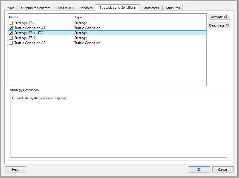
This tab presents a list with all the strategies and traffic conditions defined in the model. Those which are ticked in the list will be taken into account in the simulation of this scenario. Also, for each strategy or traffic condition, you can add a description in the Strategy Description text box below.

See the Traffic Management section for more information about using strategies.

Parameters Tab

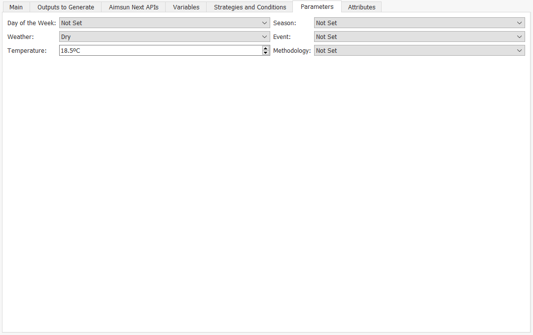
On this tab you can select information about the scenario from six fields, all of which are drop-down lists except for Temperature:

• Day of the Week
• Season
• Weather
• Event
• Temperature (range is -15°C to 20°)
• Methodology

Except for Weather and Temperature, this information is purely descriptive and is not used in the simulation. Weather is used if the MFC model is activated for any vehicle (for more information, see MFC model). Temperature is used by the Battery Consumption Model when it is activated for any vehicle (for more information, see Battery Consumption model).

Experiments

An Experiment is the object that customizes and runs a simulation scenario. Multiple experiments can be created for a scenario.

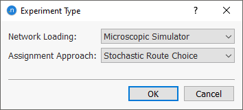
To create a new experiment, in the scenario context menu, select New Experiment and select the simulation method, meso, micro, hybrid meso–micro or hybrid macro–meso and the assignment method SRC or DUE.

The Experiment context menu has options to remove, rename, or open the Experiment properties editor.

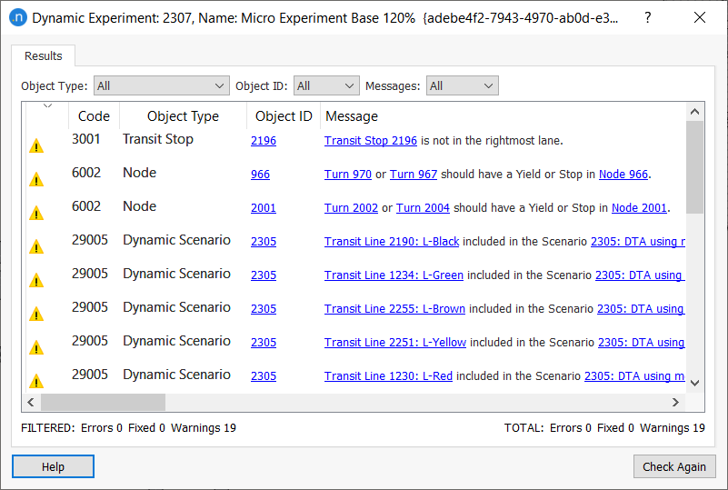
The Check and Fix Experiment option is used to check the model and the conditions for the experiment. Clicking on the hyperlinks in the report will open the properties editor for the relevant object where the issue can be rectified.

The Mark Traffic Management Locations option identifies those locations where traffic management actions are in force. This can be filtered by time of day to focus on specific actions.

The context menu also has options to run the experiment. For a dynamic experiment this first requires Replications and Averages are added to it. For a static experiment, where there is no need to run multiple replications there is a single option to run the experiment.

Dynamic Experiment Editor

The Dynamic Experiment editor has several tabs; their presence or not depends on the experiment type. The tabs are:

• Main tab: Common to all dynamic experiment types, the DUE option includes assignment convergence parameters.
• Behavior tab: This includes car-following, lane-changing and queueing behavior parameters in micro experiments, simplified behavior parameters in meso and hybrid macro–meso experiments, and all in hybrid meso–micro experiments.
• Reaction Time tab: This includes reaction time settings for micro and meso behavior, or both in meso–micro hybrid experiments.
• Hybrid tab: This is specific to hybrid experiments only (meso–micro or macro–meso).
• Dynamic Assignment tab: This is specific to experiments with a traffic demand based on OD matrices. Depending on the experiment type, either the Stochastic Route Choice or Dynamic User Equilibrium subtab is also present.
• Arrivals, Variables, Policies, and Attributes tabs: These are common to all experiment types.

Main Tab

The Main tab is used to select which pedestrian simulator to use (if relevant), to set the Initial Simulation State parameters, to include or exclude any Attribute Overrides, to specify Performance Settings, and to select any Pre-Run or Post-Run scripts required to support the simulation.

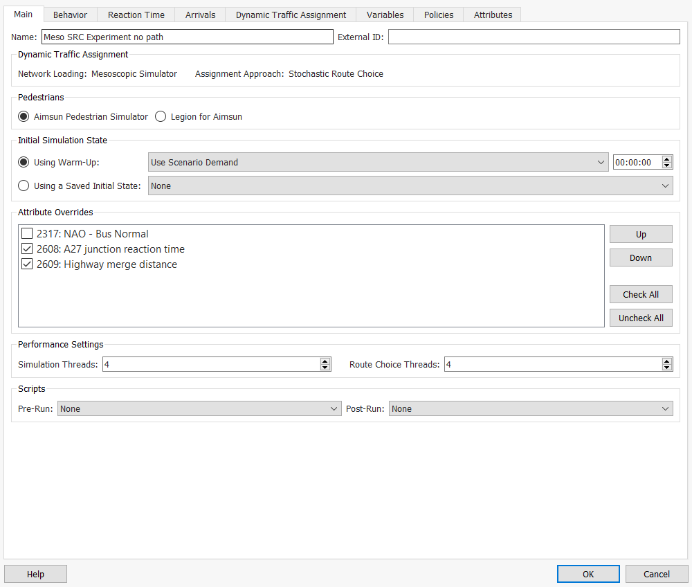
Dynamic Traffic Assignment

This information panel describes the method of network loading (e.g. micro, meso, hybrid, etc.) and the assignment approach (e.g. stochastic route choice or dynamic user assignment).

Pedestrians

If your simulation models pedestrians, you can choose one of two pedestrian simulators to use. Click on their names below for more information about when to use them.

• Aimsun Pedestrian Simulator (our built-in simulator)
• Legion for Aimsun (an external simulator licensed by Bentley Systems)

Initial Simulation State

The initial simulation state addresses an issue in microsimulation, hybrid, and mesoscopic simulation where at the start of the simulation, the network is empty of vehicles and hence will be unrepresentative of the traffic conditions until vehicles are at all stages of their journeys, including arrival at their destinations. The initial simulation state loads the network either by running the simulation for a warm up period, or loading a snapshot of vehicles from an earlier simulation. The options to load the network prior to the simulation start are:

• Select a warm-up period. The options are to use the Scenario Demand or another Traffic Demand to define the demand during a warm up period. (which should be comparable to the longer journeys in the traffic network to allow vehicles to reach their destinations) The Scenario Demand is taken to be the same as that defined in the first time slice in the scenario.

• Select a previously saved Initial State.

• An initial state can be taken from a simulation which stores the vehicles at a chosen time. To store an initial state, halt the simulation and use the context menu to store the state.The states are stored in the Project: Demand data: Initial states folder and can be renamed to identify them. It is also possible to automatically store an initial state at a predefined time during the simulation.

• In a mesoscopic simulation an initial state derived from a previous mesoscopic simulation can be used. In this case, only the automatic option is available. See the mesoscopic initial state section for more details.

During the warm-up period, the simulation uses signal controls in the master control plan when it is defined to run before the simulation start time. If the master control plan is not defined before the simulation start time, then the signal controls defined for the first period of the simulation will be used. Transit warm up however does require a transit plan that extends back into the warm up period to generate buses in that time.

Attribute Overrides

The Network Attribute Overrides defined in the project are listed. Those applicable to this experiment can be selected here and the order that they are applied edited.

Performance Settings

Aimsun Next offers the possibility to make the best use of the power of the computer when it has more than one CPU. In this case, Aimsun Next can run the simulation in parallel achieving a better execution time for each replication run. The parameters are:

• The number of threads to be used to simulate vehicle movements.
• The number of threads to be used for the route choice calculations.

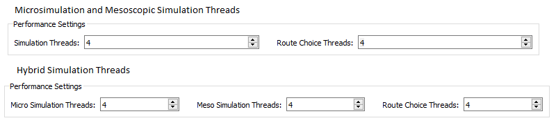
The maximum number of threads should not exceed the maximum of the number of threads in the software license or the number of threads supported by the computer being used. In all cases, microsimulation, mesoscopic simulation and hybrid simulation, the maximum number can be used for both the simulation and the route choice calculations as these calculations occur at separate stages of the simulation. Furthermore, in the hybrid meso–micro case, the maximum number can also be used for both the mesoscopic simulation and the microsimulation vehicle movements.

Note that the performance characteristics do not necessarily scale linearly with the number of threads and in small networks the overhead in using threads to parallelize the calculations might exceed the benefits of parallelization. In large networks however, the execution time will be reduced.

The default license conditions are that users with a Pro Micro Edition, a Pro Meso Edition or an Advanced Edition license can use up to four threads. Users with an Expert Edition license can use up to eight threads. If more threads are required, then the license can be extended.

Scripts (Pre-Run and Post-Run)

Scripts can be defined to be run before the execution of an experiment and after the execution of an experiment. These are set in the Pre-Run and Post-Run selectors.

There is a mandatory requirement that both these scripts must contain the following function to check any prerequisite the script might have. This function will return True if the experiment can be run or False if something is missing or invalid (the run will then be canceled). The signature of the function is:

def filter( experiment ):

    ...
    return True

Hybrid Tab

The Hybrid tab mainly contains areas to be considered micro in a Meso–Micro Hybrid and meso in a Macro–Meso Hybrid. Note the Behavior Tab also includes both micro and meso options as well as the hybrid options if a hybrid meso–micro experiment is used.

Microsimulation Scope

The Microsimulation Scope section is used to specify which simulation areas are to be microsimulated in the experiment. There are some predefined rules that can be used to add more sections and nodes to the microsimulation areas which are selected in this tab:

• Sections ending on nodes featuring an Actuated Signal Control Plan.
• Sections ending on nodes featuring a Bus Priority Signal Control Plan.
• Sections featuring a Stop for any Transit Line in use.
• Sections ending on nodes with a Controller and/or a controlled Detector or Pedestrian Walk.
• All Sections included in any Transit Line in use.
• Sections containing a Detector featuring Equipped Vehicles detection.

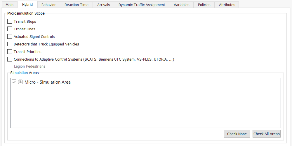
In all these cases the same rules are applied as used when considering microsimulation areas. If a section is set to be simulated as micro then the destination node and then all sections ending at this node are also set to be simulated as micro.

Mesosimulation Scope

The Mesosimulation Scope section is used to specify which simulation areas are to be mesosimulated in the experiment.

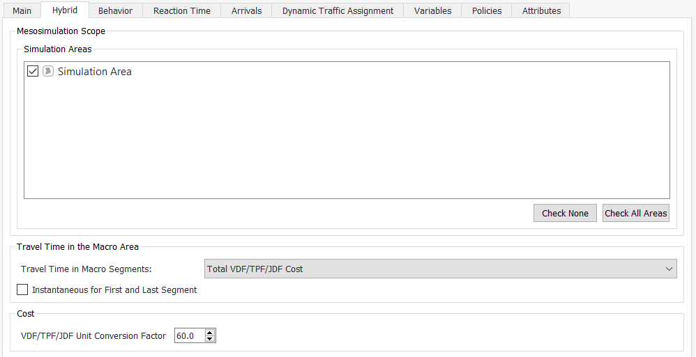
Other parameters that need to be specified:

• Travel Time in the Macro Area: there's several options to calculate it:
  • Total VDF/TPF/JPF Cost, where the travel time for each macro part of the trip corresponds to the addition of the values of macro costs in sections and turns.
  • Function Component, where the user will select an available function component that returns travel times for sections and turns.
  • Instantaneous for the First and Last Segment. When this option is toggled on, if the first and/or the last segment of the trip are macro, vehicles will appear directly in the first meso part and disappear immediately after the last meso part of the trip, and travel time for these two parts will not be computed.
• Cost Conversion Factor to transform the units of Macro costs functions to the units used in the Dynamic cost functions.

Behavior Tab

The Behavior tab controls dynamic vehicle behavior and is context sensitive depending on the simulation mode selected, micro, meso, or hybrid.

Microscopic Behavior

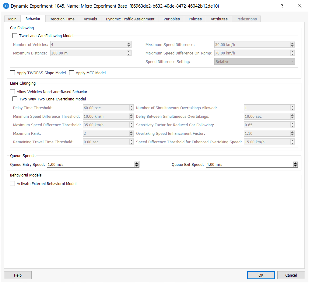
In this tab, you can define the global parameters to be used in the Two-lane Car-Following model, the Two-Way Two-Lane Overtaking Model, the Non-Lane-Based Behavior and the Queuing Speeds.

You can also choose to activate the TWOPAS slope model calculation or the MFC model if either of these is required.

If the simulation is to consider pedestrians, you can also activate the Dynamic Transit Assignment.

Furthermore, any parameters for external behavioral models developed using the microSDK (which requires a microSDK license) will be included here.

Mesoscopic Behavior and Macro–Meso Hybrid Behavior

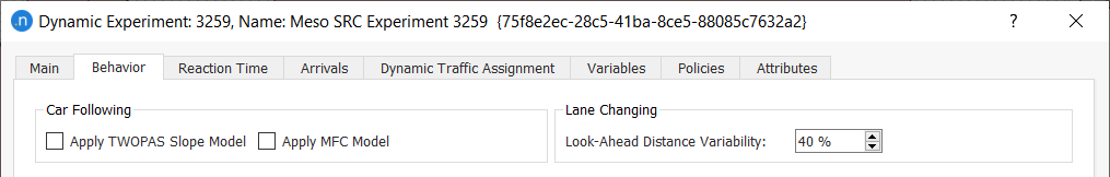
In a Mesoscopic or Macro–Meso Experiment, only the meso lane changing and the meso car following models are applicable.

Meso–Micro Hybrid Behavior

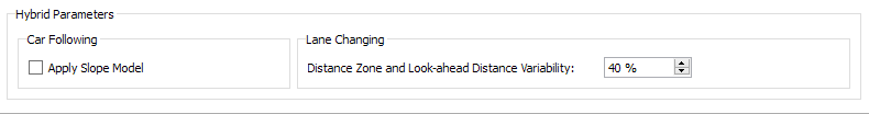
In a Meso–Micro Hybrid experiment, in the Behavior tab a Hybrid Parameters section is available to edit parameters which control the mesoscopic model in addition to the microscopic parameters applied in the microsimulation areas.

Reaction Time Tab

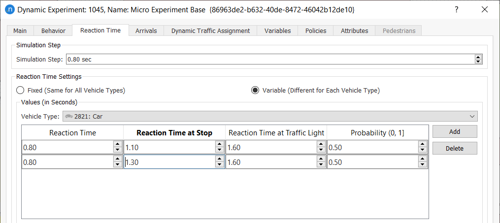
This tab defines the simulation step for micro and hybrid meso–micro simulations and the reaction times, including the reaction time at stop and reaction time at traffic lights for micro, meso, and hybrid simulations. Refer to the Global modeling parameters - General Section for details about the Reaction Time parameters.

The reaction time can be defined as Fixed, that is, the same as the simulation step or as Variable. When Variable is chosen, a list of reaction times for each vehicle type can be defined by selecting the vehicle type and using the add and delete buttons to create a reaction time profile. Each vehicle sets its reaction times using the probabilities attached to the profile.

Arrivals Tab

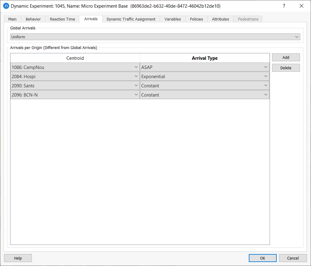
This tab controls the headway between consecutive vehicles as they arrive at the entry points in the network. The Traffic Demand sets the number of vehicles which will arrive in a time period, the arrivals algorithms control how they are distributed within that time and the time interval between them.

The time interval between two consecutive vehicle arrivals is sampled from a random distribution, six different headway models are available:

• Exponential (default)
• Uniform
• Normal
• Constant
• ASAP
• External

The arrivals model is set for the experiment but can be overridden for individual centroids for OD traffic demand, or for individual sections where demand is controlled by traffic states. Use the add and delete buttons to edit the list of overridden arrivals and select the centroid and the arrival type from the drop down lists.

The details of the arrival types are in the Arrivals Section.

Dynamic Traffic Assignment Tab

The Dynamic Traffic Assignment Tab specifies the parameters for the Stochastic Route Choice option or the Dynamic User Equilibrium option depending on the type of experiment chosen.

The common parameters to both DUE and SRC assignments are set in this tab.

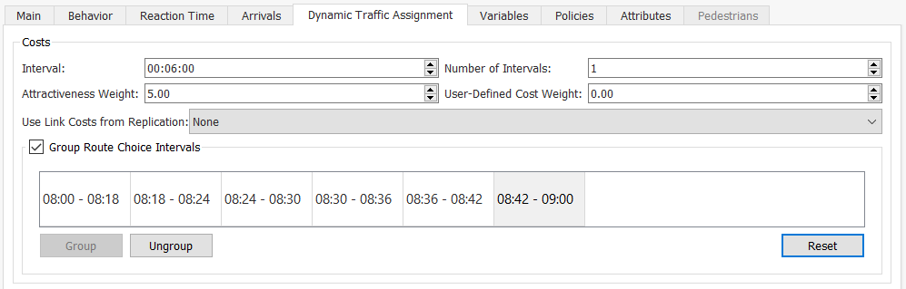
• Interval. This parameter defines the time interval t used in the dynamic traffic assignment algorithm and it defines the interval between recalculations of the shortest path.
• Number of Intervals. When the dynamic cost function of each link is evaluated, the data is derived from the previous intervals defined by the interval time. The number of intervals is configurable. A value of 1 means the link times are taken from the previous interval only, higher values take data from further back in simulated time. A short interval time and a low number of intervals could lead to path costs instability, a long interval time, and a large number of intervals to a lack of responsiveness to changes in congestion.
• Attractiveness Weight. This is a user-defined attractiveness weight parameter that allows the user to control the influence that the link attractiveness has on the cost in relation to the travel time (see link cost functions section)
• User-Defined Cost Weight. This is a user-defined cost weight parameter that allows the user to control the influence that the section user-defined cost has on the total link cost.

In a DUE experiment, you can choose a Path Cost parameter of Instantaneous, Experienced, or Time-Dependent.

• Instantaneous: path costs are calculated by adding the link costs of the path collected over the last n intervals
• Experienced: path costs are calculated by using the cost experienced by vehicles assigned to the path and that have completed the path in the last n intervals.
• Time-Dependent: path costs are calculated using the time interval in which the path uses each link, which depends on the departure interval when a vehicle was first generated in the network plus its accumulated travel time to the link whose cost is being calculated.

The Time-Dependent shortest-path (TDSP) calculation finds the least-cost route from an origin to a destination while taking into account the fact that the cost for a vehicle to traverse a link changes over time.

This method is the obverse of the instantaneous shortest-path calculation in which the cost of the departure interval is used for all links in the path.

TDSP is best used in networks where the majority of trips take significantly longer than the route-choice interval to reach their destinations, and in which congestion changes significantly over time. Large-scale models that cover peak periods tend to meet these conditions.

In such cases, TDSP calculates better paths than both Instantaneous and Experienced costs. However, if you have models that already use the Experienced option, you might prefer to continue using this cost at first. However, we consider it to be a legacy option and will eventually discontinue it.

Note: Our algorithm provides an exact solution only when the only time-dependent cost component is travel time. If the cost function contains other time-dependent components, such as attractiveness or toll charges that change over time, we cannot guarantee least-cost paths. In most cases this problem doesn't arise but it is worth bearing in mind in case of convergence issues in the DUE.

In an SRC experiment, there is an option to take the costs from a prior replication, possibly from a different experiment.

Group Route Choice Intervals

The interval time for the route choice intervals gives a basic division of the simulated time into a set of regular intervals and the path costs are recomputed at the end of each interval. The need for this recalculation might, however, vary over the modeled period. The changes in path costs, and hence path choice, will be higher in times of peak congestion while, in the same model, the changes in path cost in off peak periods will be less, with correspondingly few changes in path choice.

The Group Route Choice Intervals option allows route choice intervals to be grouped and the path costs evaluated at less frequent intervals when there is less variation in congestion and hence less need to recompute path costs and vary path choice.

In the example below, the interval time is set to 6 minutes. The first 3 intervals have been joined, as have the last 3, the paths are therefore evaluated at 08:00 as the simulated period starts, at 8:18 and then every 6 minutes until 08:42 when the last 3 intervals are merged.

Fixed Routes

For each vehicle type defined in the traffic demand the percentage of predefined (user-defined) OD Routes usage can be defined. If this percentage is set to 0 then only paths calculated by the SRC or DUE process will be used, otherwise the percentage of vehicles for all OD pairs with OD routes defined will use the fixed OD routes previously defined.

In addition, for SRC experiments (see the Stochastic Route Choice: initial assignment section), if a Path Assignment Plan has been selected in the Scenario inputs, the percentage ‘Following Path Assignment Results’ determines the probability of a vehicle following the APA files (after having substracted from the demand vehicles following OD Routes).

OD Route percentage is the first value considered as a vehicle enters the network. If the probability determines that the vehicle is assigned with an OD Route, then Aimsun Next will look for a path according to percentages and routes defined in the OD Matrix: Path Assignment folder. If the vehicle is not assigned to any OD Route, then in SRC experiments the probability of being assigned according to a Path Assignment Plan is applied (assuming a path assignment plan was specified in the scenario inputs). Finally, if the vehicle is not assigned to an OD Route, or a Path Assignment Plan, the Shortest Path calculated by Aimsun Next (SRC or DUE models) is applied.

For example, in an SRC experiment if 60% are allocated to ‘Following OD Routes’ and 70% ‘Following Path Assignment Results’, 60% of the generated vehicles will follow an OD route, 28% (70% * (100%–60%)) will follow a path read from a path assignment plan and the remaining 12% (100%–60%–28%) will follow a path built by the route choice model. This relies on the assumption that for each OD pair there is at least a route defined in the OD Matrix Path Assignment tab folder, and at least a route in the path assignment plan.

Dynamic Traffic Assignment: DUE Sub-Tab

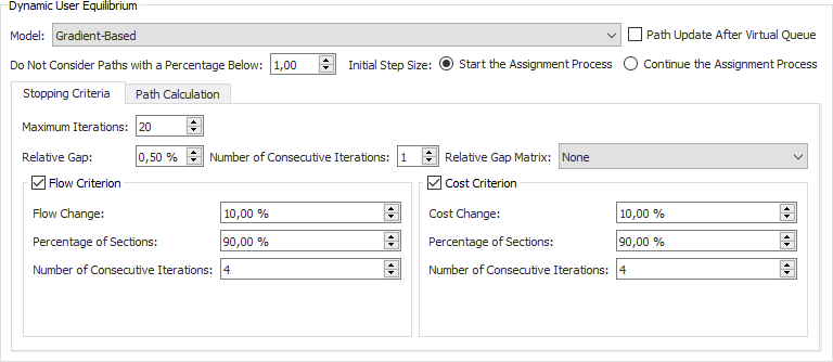
The parameters used in DUE are:

Assignment Model: This parameter defines the type of algorithm used: MSA, Weighted MSA or the Gradient-based method. These are documented in the Dynamic User Equilibrium section of the theory section of this manual.

Path Update After Virtual Queue: This parameter defines whether vehicles in a virtual queue update their path choice when a new route choice interval starts, due to a updated path assignment costs.

Do Not Consider Paths With a Percentage Below: This parameter defines the minimum percentage use that a path requires in order to be considered in the assignment. For example a percentage of 1% means that paths with an assignment percentage calculated using one of the methods defined in the Assignment model of less than 1% will be eliminated from the set of possible paths considered for the corresponding O-D pair.

Initial Step Size: If a Path Assignment Plan is defined in the scenario, then the DUE process can be started using the initial paths and path flow rates defined by that plan or it can be continued from the last iteration stored in the Path Assignment file. This option is only shown if a Path Assignment Plan has been defined. Selecting the option to continue the assignment process means that the DUE will read the Path Assignment results file and continue the DUE process that was stored in the file. To continue the DUE, Aimsun Next will first simulate an iteration using the path assignment in the Path Assignment results to have the path and link costs and then set the iteration from the file. See Start and Continue a Dynamic User Equilibrium for more details.

The different Stopping Criteria (Maximum Iterations and Relative Gap, Flow and Cost criteria and Relative Gap Matrix) parameters are described in the section on Dynamic User Equilibrium. The Relative Gap Matrix can be set in order to override the global Relative Gap and stop the paths assignment process when it reaches the relative gap defined for each OD pair. The Contents of the matrix must be set to Relative Gap and the values in the cells of the matrix are interpreted as follows:

• When the value for a given OD pair is 0, then the global value Relative Gap is used as stopping criteria for this OD pair.
• When the value for a given OD pair is greater than 0, this value is used as stopping criteria for the OD pair.

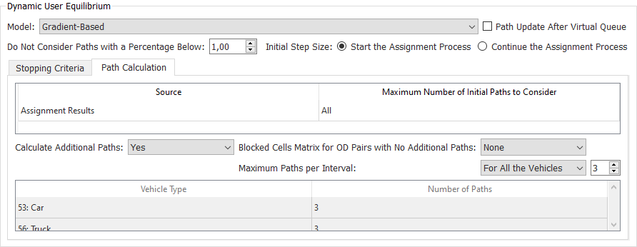
If the scenario is specified with path assignment plan, the Path Calculation is used to specify how many paths from different sources will be considered.

• Maximum Number of Paths to Consider from Assignment Results. This parameter defines the maximum number of shortest paths considered from the Path Assignment Plan files.
• Maximum Number of Paths to Consider from OD Routes. This parameter defines the number of OD routes that can be added to the set of possible routes for the corresponding OD pair. These routes and the routes calculated using the link costs will be used in the MSA or Gradient-based algorithms to calculate the path flow rates.

The Calculate Additional Paths is used to allow or prevent calculation of new paths in the assignment process and can restrict the paths assigned to be same as those in the input Path Assignment Plan. In this case the assignment process only changes the path percentages and does not include any new paths unless there was no path in the input Path Assignment Plan for a given OD pair.

There are two algorithms to calculate the paths in Meso DUE experiments: the former Dijkstra algorithm (used in all the other types of experiments) and the new A-Star model. The difference between Dijkstra and A-Star algorithms is that Dijkstra calculates a shortest path tree from one centroid destination to all sections and centroids of the network while the A-Star algorithm calculates a point-to-point path from one origin to one destination.

It's recommended to keep using Dijkstra in Meso DUE experiments when the demand is not sparse. When the demand is sparse, the A-Star algorithm will consume less memory than the shortest path trees calculation, improving the performance when running DUE simulations in large models.

The Blocked Cells Matrix for OD Pairs with No Additional Paths: option sets an OD Matrix Type with Contents: Blocked Cells. This option will prevent calculation of new paths in the assignment process but only for those blocked OD pairs defined in the OD matrix. To use this option, at least one matrix containing Blocked Cells must be created.

The Maximum Paths per Interval parameter defines the maximum number of different paths used in the path selection process applied in MSA algorithm. It can be set globally for all vehicles or set for each vehicle type.

Dynamic Traffic Assignment: SRC Tab

The general parameters used in Stochastic Route Choice are:

• Stochastic Route Choice Model. This parameter determines the discrete choice model used during the simulation. The options are: Fixed using travel times from free flow conditions, Fixed using travel times after the warm up period, binomial, proportional, logit, C-logit or user-defined and are described in the Stochastic Route Choice: Route choice model section. The Parameters will then contain parameters relevant for each of the options.

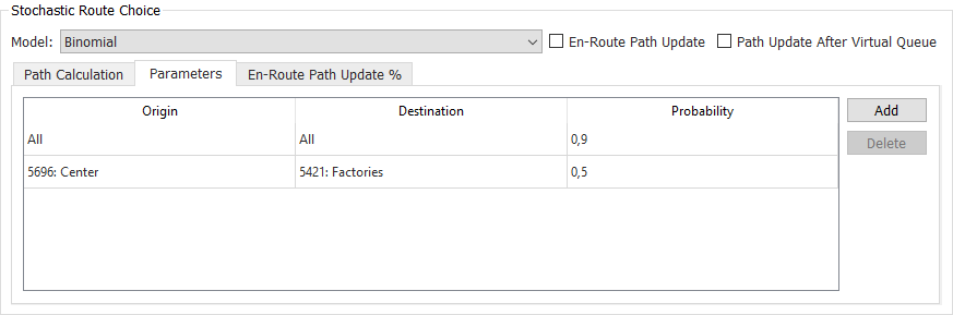
Binomial

The parameter p which controls the probability of selecting a route when the Binomial model is chosen. It is defined either for all OD pairs, but can be also specified for particular OD pairs. In the example below, the probability p assigned to all OD pairs is 0.9 except for one, where the probability p assigned is 0.5.

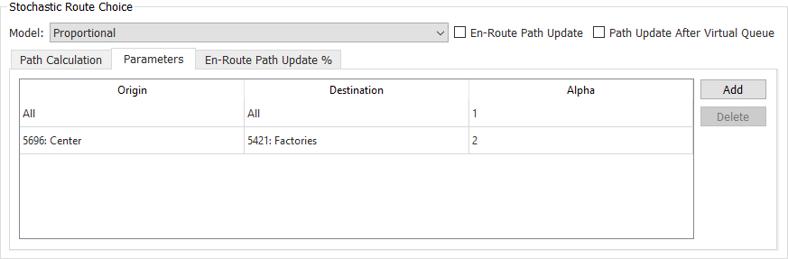
Proportional

The alpha factor parameter, alpha value can be defined via the Route Choice parameters window when the Proportional model is selected (see next figure). In this example, the alpha value assigned to all OD pairs is 1 except the OD pair from origin 284 to 286 the assigned value is 2.

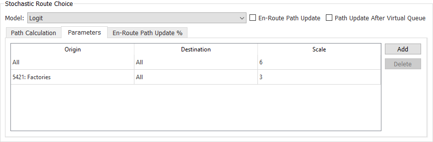
Multinomial Logit

The parameter, or scale factor, θ, is a user-defined parameter that can consequently be used to adjust the effect that small changes in the travel times might have on the driver’s decisions. The scale factor parameter can be defined via the Route Choice parameters window when the Logit model is selected. In the example here, the value assigned to all OD pairs is 10 except the OD pair with origin 288 and destination 288 where the assigned value is 5.

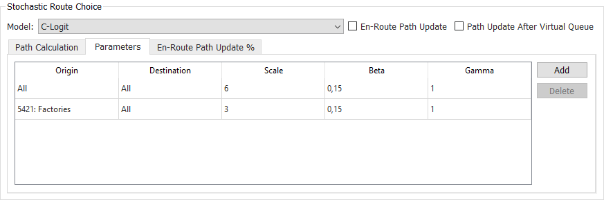
C-Logit

The scale factor parameter, θ, and the commonality factor parameters, β and γ, can be defined via the Route Choice parameters window when the C-Logit model is selected (see next figure).

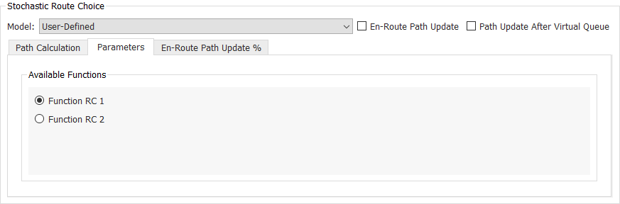
User-defined Route Choice Model

As an alternative to the default Route Choice Models, User-defined Route Choice Models can be used. Selecting the "User-Defined" Route Choice option in the Parameters tab displays a list of user-defined Route Choice functions available.

En-Route Path Update: When checked, this option allows an en-route path assignment update. When this option is enabled then the subtab folder “En-Route Path Update %” is activated which defines, for each vehicle type, the percentage of vehicles that follow a specific path type (OD routes, Path Assignment Plan or calculated shortest path) and can apply en-route path updates. These vehicles will be considered as guided vehicles.

Path Update After Virtual Queue: When checked, this option allows a path assignment update for all vehicles waiting in a virtual queue. This action will be done for all vehicles in the virtual queue independently of the En-Route Path Update %.

Use Link Costs from Replication: The link costs for the Stochastic Route Choice can be taken from another experiment or from a replication in the same scenario.

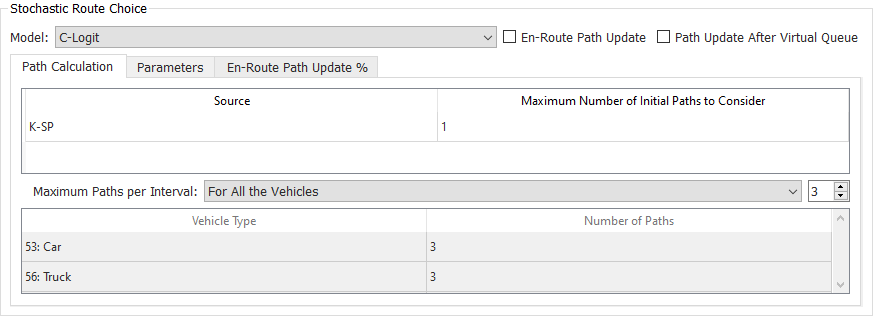
The parameters in the Basic are:

• K-SP. This parameter defines the number of shortest paths calculated at the beginning of the simulation. If this parameter is equal to 1, only one shortest path tree is calculated per destination centroid at the beginning of the simulation, taking into account the initial cost function. Otherwise, it calculates the k shortest path trees.

• Maximum Paths to Use from Input Path Assignment Results. This parameter defines the maximum number of shortest paths considered from the Path Assignment Plan. The paths used will those with the highest assigned percentage of flow.
• Maximum Paths per Interval: This parameter defines the maximum number of different paths used in the path selection process. It can be set to the same value for all vehicle types or different vehicle types can have different number of paths.

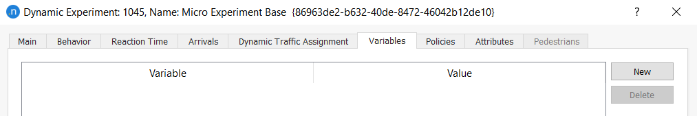
Variables Tab

The Variables tab in the Experiment Editor is identical to the Variables tab in the Scenario editor.

If the value for a variable is defined for the experiment, the value defined here will be used. If it is not defined for the experiment, the value defined by the Scenario Editor under the Scenario Variables tab, will be used.

Policies Tab

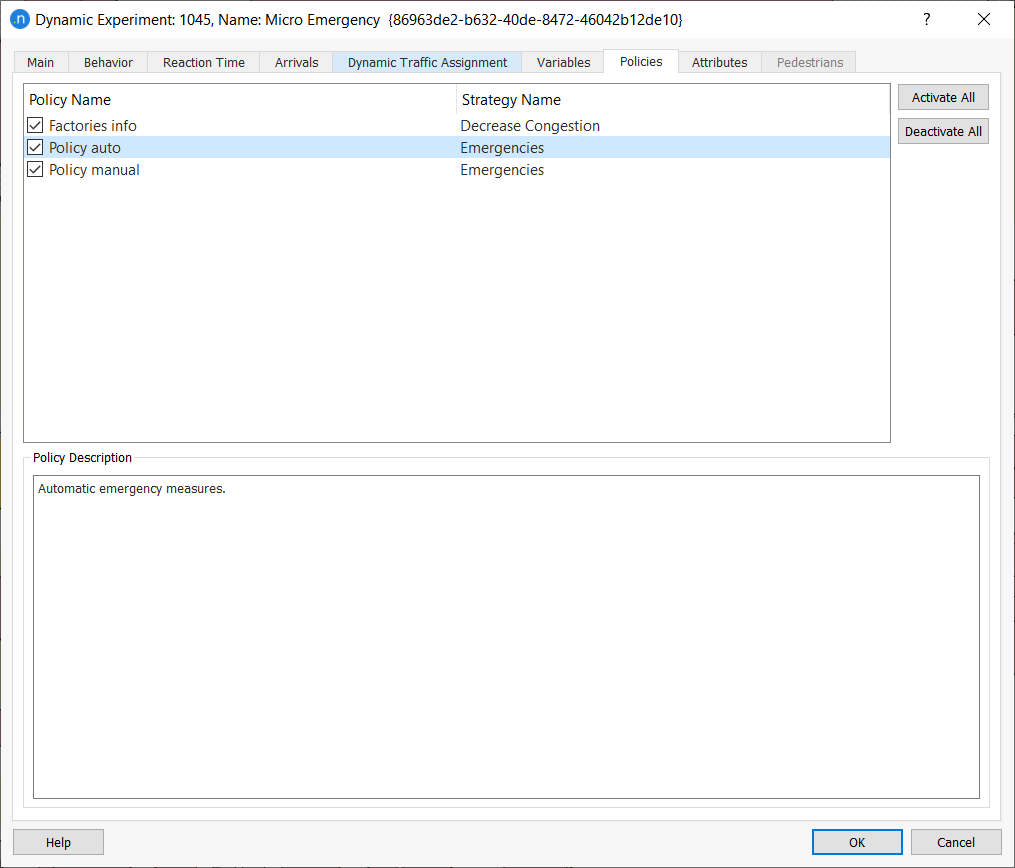
In this tab, a list of all the policies belonging to all the Strategies and Conditions that have been selected in the Scenario (in the Strategies & Conditions tab in the Scenario Editor) can be activated. Use the Activate All button to activate all policies and the Deactivate All button to deactivate all policies. Click on a policy to select it and click on an active policy to deselect it. The selected policies will be applied while running the simulation.

Policies and Strategies are described in the Traffic Management Editor.

Attributes Tab

The Attributes tab lists the attributes of the experiment.

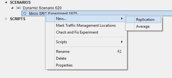
Replications and Averages for Stochastic Route Choice Experiments

A replication is the object that runs a dynamic simulation experiment once. As dynamic experiments are a Monte Carlo simulation, that is where each replication is run with a different random seed to generate different results, each experiment will therefore have a number of replications, the result of the experiment being an average of those replications.

A replication for a microscopic experiment is created using the context menu for the experiment.

The replication editor specifies the number of replications required. The number of replications is determined by the inherent variability in the simulation results and the confidence required in the average of the replications. The following advice is taken from the US Federal Highways Authority Traffic Analysis Toolbox Vol 3: Guidelines for Applying Traffic Microsimulation Modeling Software.

The required number of repetitions must be estimated by an iterative
process. A preliminary set of repetitions is usually required to make
the first estimate of the standard deviation for the results. The first
estimate of the standard deviation is then used to estimate the number of
repetitions required to make statistical conclusions about alternative
highway improvements.

The Create Average option is available if an average does not yet exist, otherwise, the Add to Average, option will appear and the new replications can be added to an existing average.

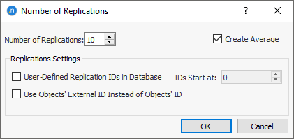
The replication IDs can be user-defined with a specified starting ID, alternately the external ID can be used to identify objects when retrieving data.

The data retrieval options for a replication are:

• Retrieve Replication Data: Loads the simulation results from an already simulated replication. In order to load previous simulations results an output source must be defined and the Store option activated (see Outputs to Generate Folder).
• Retrieve Data using an Aggregation Interval: Loads the average results from the database, but setting the interval aggregation time, which will be multiple of the current statistics interval.
• Retrieve Path Assignment Results: Loads the path assignments from the database.
• Retrieve Link Costs: Loads the link costs from the database.

Unloading Data and Results

As a complement to the retrieval options just described, to save memory, reduce computational effort, and enhance performance, there are two options that enable you to unload replication data and path assignment results from the database:

• Unload Replication Data: Unloads the replication data that were stored in the database, to save memory and enhance performance.
• Unload Path Assignment Results: Unloads the path statistics and path assignment information from the replication to save memory and enhance performance.

You might find it helpful to select one or both of these options before retrieving data and results from another replication.

Replication Editor

Once a replication is created, it can be edited by double clicking it in the Project Browser or by selecting the Properties action of its context menu.

A replication that has not been run has three tabs and appears gray in the project folder

• Main tab: Replication information.
• Outputs to Generate: To specify which outputs are generated additional to those defined by the scenario.
• Validation: To compare the outputs with observed data.

A replication that has been run has an additional four tabs and appears blue in the project folder:

• Output Summary
• Time Series
• Path Assignment
• En-Route Path Updates

The additional tabs are documented in the Outputs Section.

Replication Main Tab

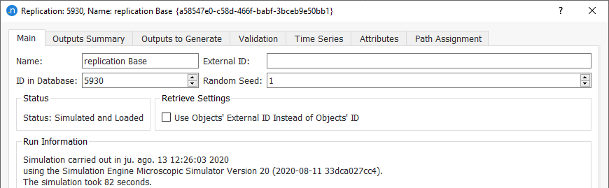
The main tab sets the replication name and whether to use external IDs instead of objects IDs to identify the objects in the database when performing retrieve data actions.

The Random Seed used by the simulator is also defined here. Each replication must have a different seed, The default seed is 0 which allows Aimsun Next to generate a unique seed for that replication. A mesoscopic simulation can use up to five extra seeds to individually control different aspects of the simulation; vehicle behavior, transit, traffic actions, path choice and vehicle characteristics. These are described in the Mesoscopic Simulation Section.

Information on the state of the simulation, whether it has been simulated or not is also supplied in the main tab

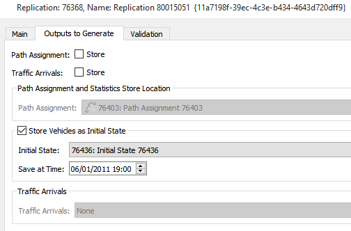
Replication Outputs to Generate Tab

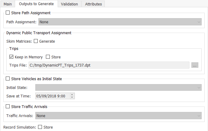
The Outputs to Generate tab is used to define additional outputs to the ones specified in the Scenario editor that will be created and filled automatically when the simulation ends. These outputs are:

• Store Path Assignment.
• Store Dynamic Transit Assignment skim matrices.
• Store Dynamic Transit Assignment trips.
• Store Vehicles as Initial State. An initial state can be selected which will be used to store vehicle information at a given simulation time. The list of all the available Initial States will be displayed.
• Store Traffic Arrivals.
• Record Simulation.

The Dynamic Transit Assignment generate and store options will only appear in this dialog provided the simulation includes pedestrians and the Dynamic Transit Assignment is activated in the experiment.

Recording and Replaying a Simulation

The Record Simulation option enables you to record a simulation for playback and review later.

To record the simulation, tick the Record Simulation option (see Recording and Playing a Simulation for more information). This copies all the vehicle positions in a replication to a file (with extension ARF) that is saved in the same directory as the Aimsun document.

The following data is recorded:

• If the replication is a microsimulation, the vehicle positions are stored every timestep and can be replayed to replicate the simulation. No interpolation to smooth the simulation is possible.
• If the replication is a mesoscopic simulation, vehicle positions are estimated and stored at a time interval specified in the replication editor. This can then be replayed and the vehicles will be displayed as dots. No smoothing is possible.
• If the recorded simulation is from the Result of a DUE experiment, then the last iteration is recorded for playback in mesoscopic or microsimulation form, according to the mode chosen for the DUE experiment.

To replay the recorded simulation, in the Project window, right-click on the replication and select Play Recorded Simulation. You might need to stop a previous simulation by clicking the x control in the task bar.

Averages

An Average is a mean of a set of replications. Averages are created using the Experiment Context Editor in the same way as Replications are created and they are edited using the context menu. There can be more than one average for an experiment and replications can be assigned to different averages as they are created or by selecting them in the Average Editor Main Tab

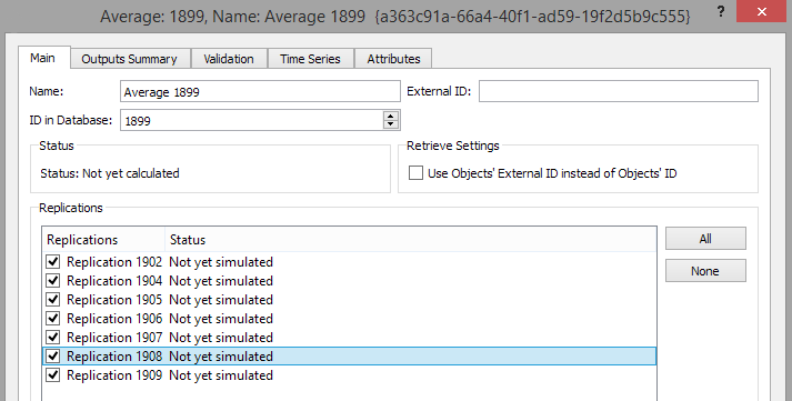
The context menu for an Average has the following options:

• Calculate: Takes the results from the attached replications and calculates the average
• Simulate Pending Replications: Run those replications that still have a Not Yet Simulated status.
• Reset Replications: Set the status to Not Yet Simulated for all attached replications, in effect forcing them to need to be re-run.

The data retrieval options for an Average are:

• Retrieve Average Data Loads the simulation results from an already simulated replication. In order to load previous simulations results an output source must be defined and the Store option activated (see Outputs to Generate Folder).
• Retrieve Data using an Aggregation Interval: Loads the average results from the database, but setting the interval aggregation time, which will be multiple of the current statistics interval.
• Retrieve Average and Replications Data Loads the average and replications results.

Results and Incremental Results for a DUE

A DUE Experiment contains one or more Result or Incremental Result which are the objects used to run the DUE experiment. Because a DUE is a dynamic experiment, the main differentiating factor between results is the random seed (or in the case of a DUE, random seeds) used to control the release of vehicles and their behavior. Other changes might include the attributes set for each different result.

A DUE can be run as a Result or as an Incremental Result, the difference is in the number of outer iterations. In a Result there is only one outer iteration using the demand defined in the scenario. In an Incremental Result there can be multiple outer iterations with increasing percentages of demand. The early iterations have lower demand which is increased at each outer iteration to 100% of the demand in the last iteration. This has the effect of running the network in an uncongested simulation in the early iterations to generate realistic route paths rather than starting in a congested situation at the first iteration.

DUE Result

The DUE Result Editor is similar to the SRC Replication Editor with an extra DUE Summary Tab that has a potential number of six subtabs to show the outputs of the DUE (the subtabs are dependent on the criteria selected in the experiment).

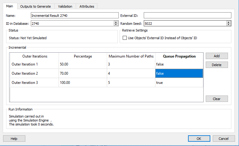
Incremental Results

In an Incremental Result, there are multiple outer iterations, these are created in the Incremental table where the proportion of demand and the maximum number of paths for each trip is specified. The convergence criteria, number of iterations and RGAP are taken from the experiment defaults. If the number of paths is not specified, the default number specified in the DTA tab of the experiment editor is used.

The Queue Propagation option in the incremental DUE controls how the network is loaded in the mesoscopic simulation. Setting this to false gives the effect of road sections with an infinite storage space.This prevents queues from propagating up into to the preceding link. This is not the equivalent of setting Jam Density to a large number, that value is still used in speed setting and in lane change calculations. Setting Queue Propagation to false gives a simulation which provides bottlenecks due to congestion as section speeds will be slow when traffic is dense, but it does not simulate gridlock as queues are not propagated back into upstream road sections. It therefore has the characteristics of a mesoscopic simulation to determine section throughputs and how congestion influences path choice while also have the characteristics of a macro assignment with no throughput constraints.

This option is used in the early outer loop iterations of an Incremental DUE with no initial paths when an AoN assignment has to be used or the demand is simply split over all available paths. This often results in over-saturation on critical sections and hence gridlock bought about by congestion due to poor path choice. Using this option avoids the gridlock, enables the assignment to complete and hence find feasible paths for the next iteration. This option should not be used in the final incremental assignment.

Using the Queue Propagation option with a reduced demand also means the DUE can be started with paths suitable for free flow conditions rather than requiring that it is warm started with paths derived from a separate macro assignment.

The remaining tabs in the Incremental Result editor are the same as in the Result Editor and the SRC Replication Editor.

Running a Dynamic Simulation

A replication can be run in Animated Simulation mode, or Batch Simulation mode.

Batch simulation does not show the vehicle animation and cannot be paused, just canceled. This is the fastest way to simulate with Aimsun Next but it offers no information about what is happening during the execution apart from the number of vehicles currently being simulated as well as the time remaining to finish the simulation. This is used to simulate already calibrated and validated experiments.

Animated simulation shows the animation of vehicles driving through the network. It is slower but it is required to observe and understand a network as it is mode and it is very useful for demonstration purposes. It is only available when running microscopic or hybrid meso–micro simulations. This type of simulation allows the simulation to be fast forwarded, removing the vehicle animation (similar to the batch mode), to be paused at any moment and the current situation to be inspected. The animated simulation is controlled using the task bar where the simulation control will appear after launching a simulation.

Note that, once an animated simulation starts, no subsequent changes made to the model will be taken into account during the current simulation. To include any changes, cancel the simulation and restart it.

Simulation Control

Once a simulation starts, you can monitor and control it by using features and tools in the task bar at the top of the 2D view.

Click the i icon on the left to see information about the replication. It displays the Replication dialog's Outputs Summary tab with an interim report on the simulation as it runs.

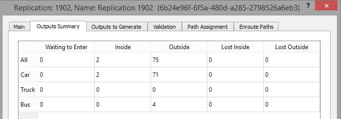
The information provided is as follows:

• Waiting to Enter: Number of vehicles that are waiting to enter the network.
• Inside: Number of vehicles that are currently in the network.
• Outside: Number of vehicles that have left the network.
• Lost Inside: If the route-based mode is in use, this shows the number of lost vehicles that are currently in the network. These are vehicles that have missed at least one of their pre-assigned turns and are now at a location from where their original destination now cannot be reached.
• Lost Outside: If the route-based mode is in use, this shows the number of lost vehicles that have left the network between the current time and the beginning of the simulation.

The playback portion of the task bar contains the following controls:

• Speed slider. This adjusts the speed of the simulation, ranging from real speed (x1), where the simulation speed imitates real time, to the fastest speed at which the computer can run the simulation, designated by the infinity icon ∞.
• Simulation date. Today's date or the date that was defined in the current scenario of the replication.
• Restart button. Restart the simulation.
• Play button. Start the simulation.
• Step forward button. Simulates one step forward.
• Fast forward button. Simulates the simulation forward as fast as possible. While fast-forwarding, you will not be able to see the animation.
• Stop button. Stop the simulation.
• Record button. Record the simulation as an AVI (video) file. See Recording a Video File for more information about recording.
• Stop At button. Click to specify a time at which you would like to stop the simulation. A new dialog is displayed where you can specify:
  • Stop date.
  • Stop time.
• Current simulation time.
• Smoothness slider. This adjusts how smooth playback appears, according to how often the animation is redrawn/updated. It has 5 positions:
  • Off: The drawing is updated every simulation step.
  • Fine: The drawing is updated approximately 10 times per second. If necessary, interpolated positions are used to achieve finer positioning.
  • Very Fine: The drawing is updated approximately 20 times per second. If necessary, interpolated positions are used to achieve finer positioning.
  • Coarse: The drawing is updated every 1 simulation steps.
  • Very Coarse: The drawing is updated every 2 simulation steps
• Cancel task button. Click X to cancel the simulation.

Note that the speed and smoothness of the simulation set in the control bar does not affect the simulation step, which is set in the experiment editor.

Recording and Playing Back a Simulation

The record and play back options enable you to review and examine vehicle behavior in detail, or to revisit a portion of the simulation from a different angle, with more visual interaction than with a recorded video (AVI) file.

They complement, rather than replace video files. In fact, you can record a video file while playing back the simulation. It works in the same way as described in Recording a Video File.

To record a simulation:

1. In the Project window, select Replication > Outputs to Generate tab.
2. Tick Record Simulation and then OK.
3. Start the simulation.

The simulation will be recorded as a rec_xxxx.arf file, where xxxx represents the ID of the replication (e.g. rec_3096). This file is saved in the same directory as the Aimsun (ANG) document.

Once the simulation is finished and the ARF file has been saved, you can replay the recorded simulation.

To play back the recorded simulation:

1. Stop any current simulation by clicking the x control in the task bar.
2. In the Project window, right-click Replication > Play Recorded Simulation.

While the recorded simulation is playing, the i icon does not appear but the functions of the task bar in replay mode are identical to the functions in simulation mode, with the exception of the Stop At button, which is not required. In addition, you can now step backward by one time step, and step forward and backward by one minute.

Note: The smoothing options are not applicable in replay mode.

If the recording was made from a mesoscopic simulation rather than a microsimulation, detailed vehicle positions are not available. Vehicle positions are estimated at the time interval specified in the replication editor and replayed at that time interval with vehicles represented as dots.

Recording a Video (AVI) File

Recording a video for any simulation is available for both 2D and 3D views for a microsimulation or a hybrid meso–micro simulation.

Note: You can also record a video while playing back the recorded simulation described in Recording and Playing Back a Simulation.

To record a video file:

1. Set your preferences for the video (see Preferences). Preferences include options for where to save the file, and characteristics like size, speed, codec, and compression.
2. In the 2D or 3D view, arrange the screen so that the video will record your desired viewpoint. You might need to select a suitable camera, zoom and pan, or change the angle to achieve the desired results.
3. Click the red Record button in the playback task bar to start the recording process. During the recording, you can also change the view to record from other cameras or to mix 2D and 3D views.
4. Click Play to start the simulation.
5. (Optional) Press the Record button again to pause the recording. Press it again to restart recording. Repeat this step as often as you require, to focus on recording certain portions of the simulation.

The image in the active view is scaled to the selected video size set in the Preferences. Make sure that you select a size that is large enough for the final video size you need.

When the recording ends or is stopped early, the video file will be available in the location selected in the Preferences.

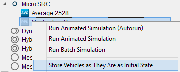
Initial States

At any time during a dynamic simulation, selecting the option to Store Vehicles as They Are as Initial State creates a new Initial State.

Simulating a Batch Replication

When simulating in batch, the task bars shows an information dialog (Click the i icon) to see a global view of the simulation while it is running. The information is:

• Waiting out: Number of Vehicles that are waiting to enter the network.
• Inside: Number of Vehicles that are currently in the network.
• Gone Out: Number of Vehicles that have left the network.
• Lost Inside: If the route-based mode is being used, the number of lost vehicles that are currently in the network.
• Lost Outside: If a route-based simulation mode is being used, the number of lost vehicles that have left the network since the beginning of the simulation.

The bar shows:

• The time taken so far to run the simulation.
• A progress bar.
• An estimate of how long is needed for the simulation to finish.
• A cancel (x) button.

Simulating a DUE

A Dynamic User Equilibrium Experiment runs a simulation multiple times adjusting the path assignments on each iteration. Each experiment is run with one random seed and the path assignment from a single simulation replication used to provide the costs inputs for the next iteration. The iterative nature of the DUE experiment reduces the reliance on results from a single seed simulation run. Users concerned about the possibility that the DUE process might converge on significantly different solutions should run multiple experiments and compare results.

While a DUE experiment is running the task bar displays:

An information dialog (Click the (i) ) for the global view of the experiment while it is running.

• The time taken so far to run the experiment.
• Which iteration is currently being simulated.
• An estimate of how long is needed for the experiment to finish.
• A cancel (x) button.

Clicking the information button brings up the Results Editor to display the simulation results.

Outputs

Scenario Output Options

The Outputs to Generate Tab in the scenario editor details which outputs are generated by the experiments in the scenario.

The statistics, paths, and relative gap matrices can be toggled on or off and the option to store the results in memory or in the database so they can be retrieved for subsequent use selected. Vehicle-based experiments can also collect detector time series data also at a specified interval. In both cases, the interval must be greater than 00:00 and smaller than or equal to the total simulation time. This will control how often the statistics are generated as the simulation runs and hence the detail in the Time Series views and in the Map Views.

Relative Gap Matrices contain the Relative Gap by each OD pair.

The Detection Cycle is the timestep at which a detector gathers information. It can be set here to be the same as the simulation timestep. In this case, the detector data will be updated at the same frequency as the simulation.

A microsimulation can also store the vehicle positions in an XML file, or in the project output database.

There are several subtabs available in the Outputs to Generate tab:

• Store Locations: Where to store output data.
• Statistics: What data to collect.
• Paths: The path statistics to collect.
• XML Animation: Storing vehicle positions in XML format suitable for input to Legion.
• Individual Vehicles: The vehicle trajectories are recorded in the database.
• Controllers: Creating Log files for signal controllers.

Store Locations

The output data for this scenario can be held separately from the project database if the Store in Database option is selected The available database options are:

• Use Project DB
• Automatic Databases (Access and SQLite)
• Custom

The database for the scenario is specified in the same way as for the project. See the Project Editor for details.

Path Assignment results are stored in a binary file with an Aimsun Next specific format (.apa). This data can also be kept in memory for efficiency The path storage options are to be found in the Replications Editor.

Statistics

The Statistics sub Tab specifies which outputs are required. These are described in detail in the Simulation Results section.

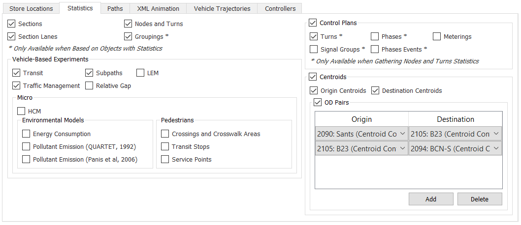
Data is available for Sections, Sections by lane, Nodes and Turns, and for Groupings of objects.

Data is also available in microsimulation and in mesoscopic simulation for transit, subpaths, and traffic management actions. The London Emission Module (LEM) outputs are available for both micro and meso simulations whereas the other environmental models are only available in microsimulation. The other microsimulation only outputs are the HCM statistics and Pedestrian outputs.

Control plan data listing when signal events occurred can be collected for turns and for signal phases and groups. The output is stored in the project outputs database.

Trip information between selected OD pairs can be gathered by specifying a set of OD pairs in the Traffic Demand box. As many trips as required can be specified by clicking the Add button, or the All option can be clicked for either the Origin centroid, the Destination centroid or both. The Origin and Demand centroid tick boxes create time series outputs per origin or destination centroid.

Paths

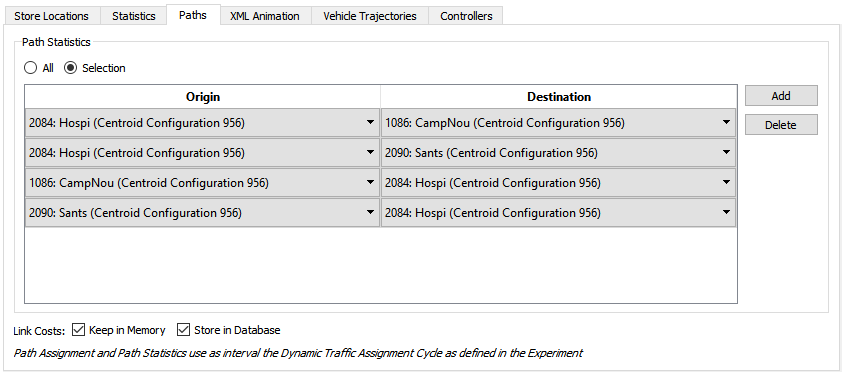
In the Paths tab, statistics for the Paths calculated by the Dynamic Traffic Assignment algorithm can be gathered. Note that this information will be only available when simulating using OD Matrices as the information is derived from the Dynamic Traffic Assignment algorithm which can only be used with OD Matrices. The interval to gather the statistics will be the same one used to recalculate the paths. Statistics can be gathered for all the OD Pairs or just for a selection; by clicking the Add button, a new OD Pair can be added and by clicking the Remove button, the selected OD Pair will be removed from the list.

Link costs can also gathered and visualized in turns statistics. The Link costs are those costs used to calculated the shortest path trees. When using OD Matrices link costs will also be displayed by the Path Analysis Tool to show the incremental costs on a path.

XML Animation Tab

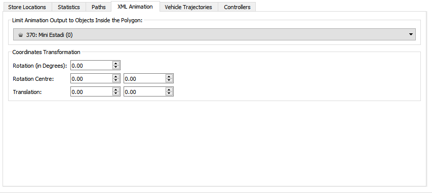
Legion Studio uses the output from an animated Aimsun Next simulation to enable pedestrian planners and engineers to include accurate simulations of roads and traffic (private and transit) in their models. By importing the XML file produced by Aimsun Next, Legion, Studio users can automate the modeling of pedestrian crossings that are synchronized with the simulation. Legion's Simulator and Analyzer uses the Aimsun Next output file to visualize traffic movement during a pedestrian simulation. Legion 3D reads the XML files along with Legion results files to produce high quality three-dimensional animations of an environment with accurate movement of vehicles and pedestrians.

If the Store XML Animation option is selected, this tab provides the ability to limit the output to those vehicles within a selected polygon and to correct the co-ordinates of the output by rotation and translation.

Vehicle Trajectories Tab

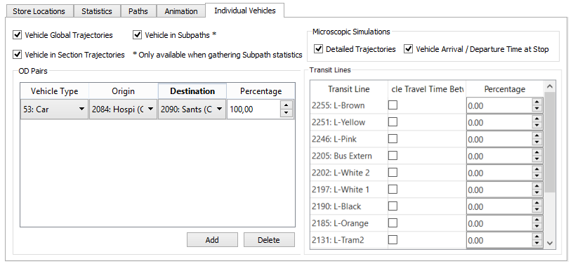
The Vehicle Trajectories tab is used to determine which of the vehicles in the simulation are selected to have their trajectories exported and what level of detail is exported. The option to store vehicle trajectories in the outputs database must be selected to enable the options in this tab.

There are three types of trajectories:

• Global trajectories: For each vehicle, the trajectory will store its origin and destination centroids. For each transit vehicle it will store the sections where the vehicle entered and exited the network. For all vehicles it will also store its entrance and exit times in the network, travel time and delay time for the whole trip.
• Trajectories by Section: For each vehicle it will store the ID of each section it has traveled though, the vehicle’s exit time from each section and the vehicle’s travel time and delay time through each section.
• Trajectories by Subpath: For each vehicle that completes a sub path, the statistics for that path are gathered and include the travel time, the number of stops and the distance traveled. The data is described in the Statistics Section.
• In Microscopic Simulations:
• Detailed Trajectories: For each vehicle, for each simulation step, it will store ID of the vehicle's current section or node, the lane index, the x and y coordinates of the vehicle’s front midpoint, the current speed, current acceleration, and the distance traveled since the vehicle first entered the network.
• Transit Vehicle Travel Time Between Stops: Information for transit vehicle trajectories regarding bus stop maneuvers, that is vehicle arrival and departure time at the transit stops.

As the amount of trajectory data can be very large, filters can be applied to limit the number of trajectories stored.

Filtering by OD Pairs

If the traffic demand selected is a collection of OD Matrices, trajectories can be filtered selecting a set of OD Pairs. Each row in the table of OD Pairs selects a set of vehicles. Only one of the rules/rows has to be true for the OD pair to be selected.

A rule/row has the following selectors:

• Vehicle Type: A specific vehicle type or “any”.
• Origin: A specific origin centroid or “any”.
• Destination: A specific destination centroid or “any”.
• Percentage: Determines the percentage of vehicles selected by this rule.

Filtering by Entrance Sections

If the traffic demand selected is a collection of Traffic States, trajectories can be filtered selecting a set of entrance sections. Each row in the table of Entrance Sections selects a set of vehicles. Only one of the rules/row has to be true for the trajectories originating in that section to be selected.

A rule/row has the following selectors:

• Vehicle Type: A specific vehicle type or "any".
• Entrance Section: A specific entrance section or "any".
• Percentage: Determines the percentage of vehicles selected by this rule.

Filtering by Transit Line

The row for each Transit Line in the Transit Plan determines the percentage of vehicles from a Transit Line that will be stored in the output database.

Controllers Tab

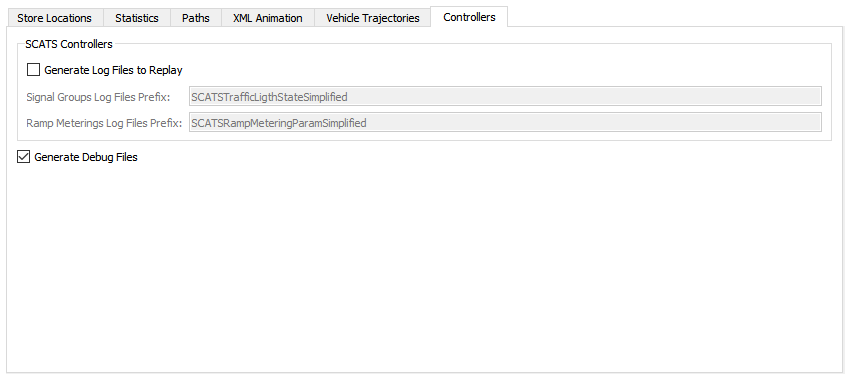
The debug output from an external signal plan controller is toggled on or off in this tab. The outputs are stored in log files in the directory (on Windows) "/Users/user/AppData/Roaming/Aimsun/Aimsun Next/Logs“. The file name is, for most controllers, AimsunNextSignalState.log, the SCATS RMS controller logs debug information to AimsunNextRampMeteringStateX.log.

Additional debug output from a SCATSim controller can be generated and subsequently used as input to a SCATS controlled junction to replay the same signals pattern, without linking to SCATSim. This is documented in the Controller Section.

Replication and Average Outputs

The properties editor of a dynamic experiment replication will be extended after the experiment has run with an Outputs Summary tab, a Time Series tab, a Validation tab and, if OD matrices were used in the simulation and a Path Assignment tab.

• The Outputs Summary tab lists the global value of all the outputs.
• The Time Series tab uses the standard time series viewer for objects to display outputs. Its use is documented in the Time Series Section.
• The Validation tab compares observed data for the scenario with simulated data from the replication. Refer to the discussion of model validation in the Calibration and Validation Section.
• The Path Assignment tab displays the path related results. This tab is only available when the Traffic Demand is OD-based.

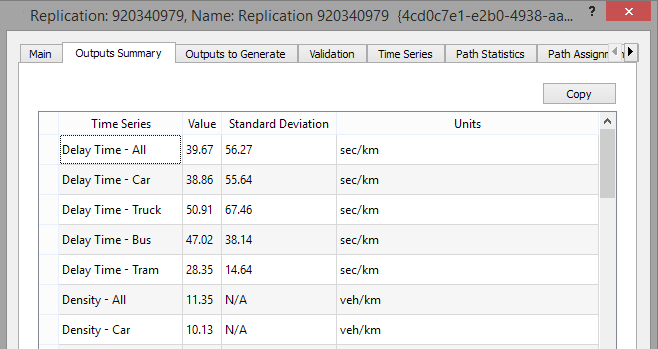
Outputs Summary Tab

The Outputs Summary Tab lists the global value of all simulation outputs with the value, standard deviation and the units. The Copy button copies the selected values in the table to the system clipboard. How these values are calculated is documented in the Calculation of Statistics Outputs Section

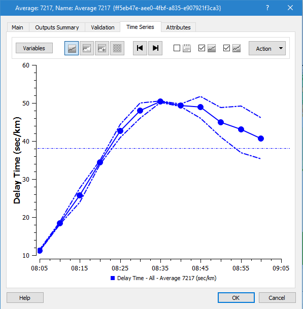
Time Series Tab

The Time Series Tab uses the Time Series Viewer to show how variables vary as the simulation runs and if multiple variables are selected, how they are correlated during the simulation. The variables listed in the time series are the global simulation measures for the replication, or the time series for a selected object can be displayed. As with all other time series displays; the standard deviation and the mean can be displayed, or the data shown in tabular form.

Validation Tab

The Validation Tab compares the observed flow or volume counted by a detector with the section flow or volume calculated in the replication. This uses a Real Data Set as documented in the Real Data Set section of the manual. The Real Data Set used in the comparison must be loaded and set in the Scenario editor:Main Tab as the Real Data Set for validation.

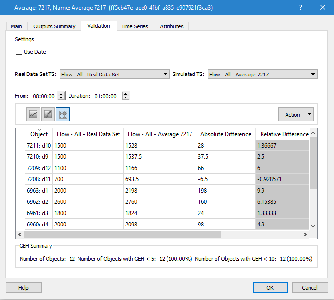
Once the corresponding Time Series to compare with the Assignment volumes is selected in the Validation folder, there are three different possible representations available: by means of a Graph, a Regression chart or a Table. These are shown in the three figures below:

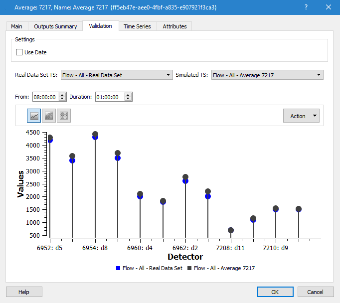
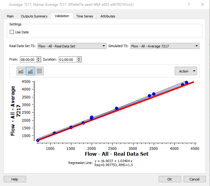
In the regression graph, the blue line is the regression line, the black lines are the 95% confidence intervals at and the red line represents the fixed line y = x.

In the table representation, the observed and assigned volumes or flows are listed, as well as their absolute difference and their relative difference computed as:

100 * ( (Assigned-Observed)/Max(Assigned, Observed))

There are also options to calculate Theil's coefficient and a GEH value.

Actions

The data can be copied as a table or as an image of the graph

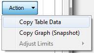
The limits of the graph can be set in the Adjust Limits option.

Path Assignment Tab

The Path Assignment Tab is described in the Path Analysis: Assignment section.

En-Route Path Update Tab

The En-Route Path Update tab is described in the Path Analysis: En-Route Path Update section.

DUE Result Outputs

The results of a DUE are similar to the results of an SRC dynamic simulation with the same paths, time series, and validation tabs. These are documented in the Replications and Averages section. A DUE result does, however, have an extra Summary tab detailing the DUE convergence.

DUE Summary Tab

The DUE summary tab has, potentially, six subtabs: Relative Gap, Flow Stability, Cost Stability, Stability, Vehicles per Iteration, and Execution Times. Which tabs appear depends on which criteria you select in the experiment. For example, if Flow Criterion or Cost Criterion are not ticked, the subtabs Flow Stability and Cost Stability will not be displayed.

Relative Gap

The Relative Gap statistic represents the difference between the current path costs and current minimum costs at each DTA interval. The Relative Gap subtab shows the evolution of the achieved Relative Gap for each DTA interval time as the process iterates. The interval time is set in the Experiment Editor DTA Tab.

In an Incremental Result, the Relative Gap for the last outer iteration with 100% of traffic demand is shown.

Stability Subtabs

The Flow Stability and Cost Stability subtabs show, for each path calculation interval, the percentage of links whose flow/cost variation (with respect to the previous iteration and the same interval) are below the value required as a stopping criterion.

For each iteration, slice, vehicle type, and link, the count and costs, as well as the variation of these compared with the previous iteration, can be seen in the Stability subtab.

A Note on Flow and Stability

In flow-stability and cost-stability graphs, when an interval reaches convergence (when stopping criteria are met) its percentage value is retained in the graph for any iterations that follow. For example, the dark blue line for interval 08:00:00 in the graph below reaches convergence at iteration 6 and its value remains the same for iterations 7–13.

In actuality, once an interval has converged, the distribution of vehicles is stopped, meaning that the real variation is zero from that moment. However, we maintain the values in the graph so that you can see the percentages that every interval needed to reach convergence.

However, on the Stability subtab, the real cost and count data are reported. Therefore, for all iterations of an interval following the one where convergence was achieved, 0% variation is recorded, as can be seen in the Count Variation and Cost Variation columns pictured below.

You can find more information about convergence in the Convergence Criteria section of the theory section of this manual. Note that they are stored in the database as raw data: count and cost by section, by iteration, by slice, and by vehicle type (see also DUE Convergence Tables).

Vehicles per Iteration

The Vehicles per Iteration subtab shows:

• Waiting to Enter: Number of Vehicles that are waiting to enter the network.
• Inside: Number of Vehicles that are currently in the network.
• Outside: Number of Vehicles that have left the network.

Execution Times

The Execution Times subtab shows for each iteration, in seconds:

• DNL: Time for the Dynamic Network Loading. This is the time of the simulation.
• SP: Time for the shortest path calculation.
• MSA: Time for the Method of Successive Averages algorithm.
• RGap: Time for the calculation of the Relative Gap.

Global Execution time (in seconds): The mean of the times for each iteration, and a running total of simulation time.