Dynamic Traffic Assignment Algorithms

For Dynamic Traffic Assignment, the traffic demand is defined in terms of OD matrices, each one giving the number of trips from every origin centroid to every destination centroid, for a time slice, and for a vehicle type. When a vehicle is generated at its origin, it is assigned to one of the available paths, connecting this origin to the vehicle’s destination. These paths are computed as the simulation starts and recomputed at the route choice time interval.

The vehicle will travel along this path to its destination unless it is allowed to dynamically update the route en route (i.e. it is a guided vehicle) and a better route exists from its current position to its destination.

The simulation process based on time-dependent paths, consists of the following steps:

Step 0: Calculate initial shortest path(s) for each OD pair using the defined initial costs.

Step 1: Simulate for a predefined time interval (e.g. 5 minutes) known as the Route Choice Interval, assigning to the available paths the fraction of the trips between each OD pair for that time interval according to the selected route choice model. Obtain new average link travel times as a result of the simulation.

Step 2: Recalculate shortest path, taking into account the new average link travel times.

Step 3: If there are guided vehicles, or variable message signs which suggest a change of route, provide the information calculated in step 2 to the drivers that are dynamically allowed to update path en route.

Step 4: Go to step 1.

This section describes:

• Road Network Representation: Describing how the route choice network is represented.
• Defined Paths: These are fixed paths supplied by the user or from another experiment.
• Link Cost Functions: Describing how the perceived cost of traversing a road section is derived.
• Routed Paths: Describing how route paths are found.
• Path Selection: Describing how vehicles choose their paths through the network including the effect of information from ITS systems to cause vehicles to update path choice en route.

Road Network Representation

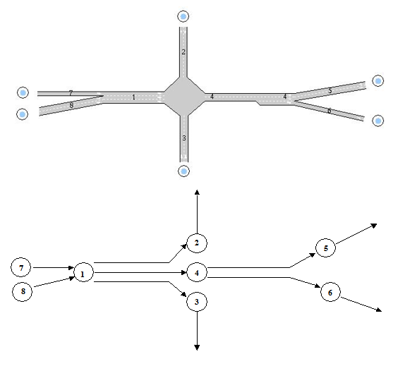
The use of sections and intersections, the network representation used for the microscopic simulation, is inappropriate for the path computation algorithms. This requires a link-node representation which explicitly accounts for turn movements at the end of a section and therefore, the link that connects two nodes used in route choice calculations will contain both a section and a turn movement.To convert from a road section and intersection representation to links, each road section is split into the same number of links as there are turn movements at the end of the section; each link can then be assigned a cost of traversal which includes the cost assigned to the turn at the end of the link.

The next figure shows an example of a traffic network composed of sections, junctions, and joins. The corresponding network representation used by the route algorithms, composed of nodes and links, is shown below it. Note that, for each section, a node is created and there is a link for each turn movement. The cost assigned to each link is a function of the travel time of the section plus the travel time of the turn movement.

Defined Paths

The paths available from an origin to a destination, which are taken into account in the path selection process for the vehicle, can either be defined by the user (user-defined routes or user-defined path trees) or calculated by applying a shortest path algorithm, which uses the concept of “cost”.

OD Routes (formerly known as User-defined routes) correspond to the idea of well-known paths, or the most familiar paths for drivers, from an origin to a destination according to the analyst’s knowledge of the network being modeled. They are predefined by the analyst using the network editor or taken as an output from other traffic simulators or transport models, whether macroscopic or microscopic.

Path Assignment Routes from an assignment experiment are the result of applying a static traffic assignment using Aimsun Next macro or a dynamic traffic assignment based on dynamic user equilibrium using microsimulation mesoscopic simulation. These paths correspond to OD Routes, the difference is in their representation. The OD Routes are a list of links from one origin to one destination while the paths derived from an Assignment result have a structure which defines a path from each link on the network to one destination. The two structures, from logical point of view, represent a point to point path, but in the first representation, OD Routes, when a vehicle loses a turn movement, it loses its path and there is no way to recover it. However, with the paths derived from an Assignment result, the vehicle can continue its path from the new link.

Shortest paths are calculated by applying the shortest path algorithm to a network represented as links and nodes, in which each link has an associated cost function (i.e. travel time) that will provide the cost used in the shortest path calculation. The costs can be calculated using the Initial Cost Functions or by using the Dynamic Cost Functions depending on the choices made in the traffic assignment calculations.

Link Cost Functions

In the link-node representation of the network used in calculating the shortest routes, a cost function is associated with each link. Three types of link cost functions are used to calculate the shortest path, depending on whether simulated data (i.e. simulated travel time) are available or not, they are the K-initials shortest path cost function, the initial cost function and the dynamic cost function. In all three cases, there is a default cost function, which represents the link travel time in seconds composed of a section travel time plus the turn movement travel time; this last term introduces the time penalty of the turn movement at the end of the link.

Link cost values have a range of possible values [1e-06..1e06]. All values outside this range are replaced, values lower than 1e-06 are replaced by 1e-06 and values higher than 1e06 are replaced by the maximum cost in the range times 10.

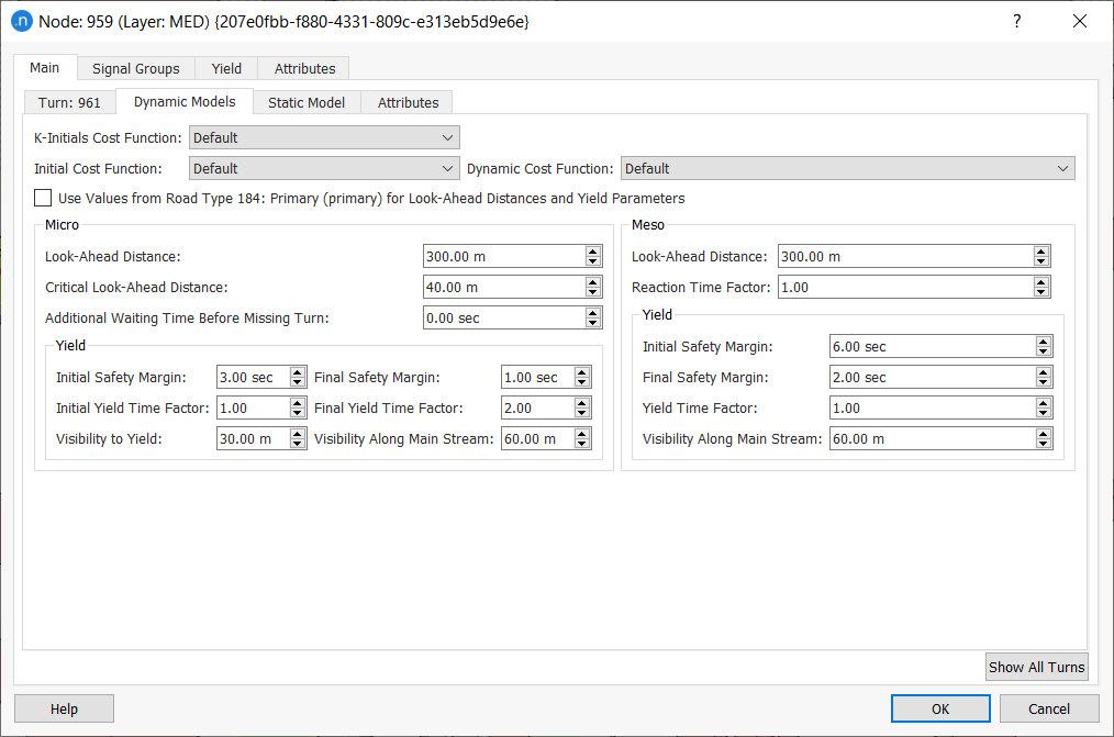
For each link, the user can choose between using the K-Initials Shortest Path Cost Function, Initial Cost Function or Dynamic Cost Function, the default cost function (selecting Default), or using any other cost function defined by the user. This is selected from the Cost Functions list box of Edit Turn tab in the Node Editor, the cost function parameters are described in the turn as the turn is the unique object that differentiates links that share the same road section.

Note the K-Initials Shortest Path Functions are used only when the K-Initials Shortest Path calculation is used.

The list of cost functions available, and how these are created and edited, is described in the Cost Functions Section

Link Attractiveness

The attractiveness of a link can be set in the Node editor on the Turn subtab and it will apply to all routing links which include the affected section.

However, the network can calculate an automated attractiveness value which is based on several elements: the theoretical flow capacity of the origin and destination sections, the number of lanes in the sections involved, the number of turns with the same origin section, and the theoretical flow capacity of these turns.

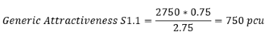
A lane can have a weight that denotes its contribution to the calculation of the capacity of a link. For example, a central lane makes a complete contribution to the capacity of a link and therefore has a weight of 1. However, an exit or a side lane has a smaller weight of 0.75. So the weight of a lane (WL_i) is defined as 1 for a central lane and 0.75 for side or exit lane.

The generic capacity per lane in a section s is therefore defined by:

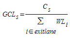
where C_s is the capacity of section s.

Attractiveness Algorithm

The attractiveness of a link – a link being a section (s) plus a turn (t) – is obtained as a result of an algorithm which performs the following five steps:

1. For each turn being considered, it finds the desired attractiveness of every turn that leaves the origin section s (this can be the capacity required by destination lanes or the manual capacity set by the user in t itself).

   Desired attractiveness is the theoretical amount of attractiveness that a turn would have if the capacity of the origin section (s) were infinite. But the origin's capacity is always finite and might be smaller or larger than the desired attractiveness. For example, the destination section might request 1,000 PCUs and the origin lane might be able to supply 500 PCUs, or even 2,000 PCUs.

   In these cases, the destination would receive 500 and 1,000 PCUs respectively. This shows that desired attractiveness sets the upper bound and the origin supplies as much as it can, up to the value of the upper bound. 2. Each origin lane has a capacity. For each outgoing turn, the algorithm subtracts the desired attractiveness from this capacity, taking the weight of a lane into account.

   The result of this calculation can be positive or negative for a lane, meaning they can either supply the desired capacity (using the lane's complete capacity or sometimes leaving spare capacity in the lane) or they have a deficit (e.g. a destination desires 1,000 PCUs but an origin can only supply 500 PCUs; this would create a deficit of 500).

   For each lane in s with GA_l (general attractiveness) the following calculation applies:
   
   
   

   where WL_i = weight of lane l

   TLW = total weight of a turn's origin lanes

2. After this calculation, the algorithm determines which lanes have capacity left over and which are in deficit (unable to supply the desired capacity). It labels these origin lanes from s as A and B:

   • Type A Lanes: this type of lane has a remaining capacity greater than or equal to 0, which is enough to provide the desired capacity from its turns and possibly have some to spare.
   • Type B Lanes: this type of lane cannot provide the desired capacity. It might need 'help' from the remaining capacity of one or more type A lanes.
3. Type A lanes redistribute their excess remaining capacity among the Type B lanes with which they share turns.

4. Any desired attractiveness that remains unfulfilled after this redistribution is corrected. This is done proportionally across affected destination lanes, using the following calculation:
   
   
   

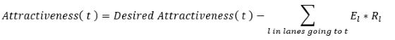
   where E_l = excess desired capacity assigned by lane

   R_l = the ratio between the assigned attractiveness by lane l to turn t and the total attractiveness assigned by l

Link cost functions should always return a value between 0.000001 and 100000. If the cost function returns a value outside this range, the value is replaced by a value that ensures paths avoid using this link. The replacement value is the sum of all link costs for a given user class, multiplied by 10. A warning is displayed in the log window for all pairs of turn + user class that don't return a cost between the predefined range.

Example Network

The illustration below shows part of an Aimsun network. It comprises four sections (1, 2, 3, and 4) and a central intersection which contains three turns. This corresponds to three links in the equivalent route-choice network. The capacity of each section is set as labeled.

Figures in blue indicate the actual capacity received by each section on completion of the five-step algorithm, taking into account redistributions of capacity and corrections.

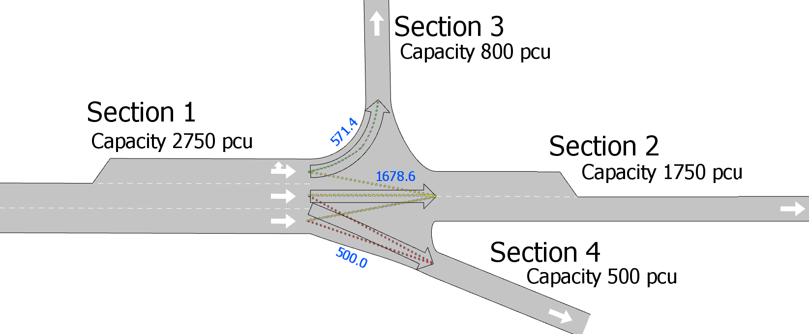
The capacities of lanes in the origin Section 1 (lanes 1.1, 1.2, and 1.3) are as follows. Note that lane 1.1 is a side lane with a weight of 0.75.

In this example, the five steps of the algorithm proceed as follows.

1. The desired attractiveness by lane is considered:

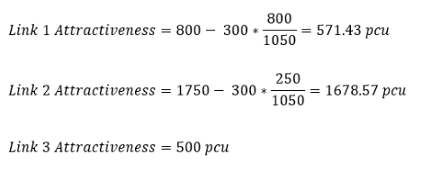
   • Link 1: S3 requires 800 PCUs from S_1.1.
   • Link 2: S2 requires 1,750 PCUs in total: 477.27 from S_1.1 and 636.36 from both S_1.2 and S_1.3.
   • Link 3: S4 requires 500 PCUs in total: 250 from both S_1.2 and S_1.3.

2. Desired attractiveness is subtracted from the lanes' capacity. The remaining capacity on origin lanes is:

   • S_1.1 = 750 – 800 – 477.27 = -527.27
   • S_1.2 = 1,000 – 636.36 – 250 = 113.64
   • S_1.3 = 1,000 – 636.36 – 250 = 113.64

3. Origin lanes are labeled as A or B:

   • Lanes S_1.2 and S_1.3 are type A lanes, with remaining capacity that can be shared with the central turn S_1.1 (a type B lane).

4. Excess capacity is redistributed to lanes with a deficit:

   • Capacity up to 227.27 PCUs that S_1.1 still needs will be shared with it by turns S_1.2 and S_1.3, leaving the following capacities:
     • S_1.1 = -527.27 + 227.27 = -300
     • S_1.2 = S_1.3 = 0

5. Any excess desired capacity is corrected.

   • This is only necessary for turns that have negative lane capacity remaining at the origin:
     
     
     

Initial Cost Functions

The initial cost function is used at the beginning of the simulation when no simulated data has yet been gathered to calculate the travel times. In this case, the cost of each link is calculated as a function of the travel time (in free flow conditions) and the attractiveness of the link. The travel time in free flow conditions is the time it would take a vehicle to cross the link, which is the section plus the turn, assuming that the vehicle is traveling at the maximum speed permitted along the section and at the maximum turn speed during the turn movement. No time penalty is included for traffic signals.

There are two types of default initial cost function: For the first type, IniCost~j~ the vehicle type is not taken into account, that is, all vehicle types have the same initial cost. For the second type, IniCost~j,vt~, the vehicle type is taken into account, which means that there is an initial cost function per vehicle type. The presence of reserved lanes in the network determines whether the initial cost function considers vehicle type or not. By default, Aimsun Next does not consider vehicle type when choosing the initial cost function, although it does consider vehicle type if there are reserved lanes.

If the penalty for turn t that belongs to the link is taken into account, the initial cost of link j, IniCost~j~, and its attractiveness, CL~j~, are calculated as follows:

where

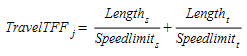
• TravelTFF~j~ is the estimated travel time of link j in free flow conditions.

• φ is a user-defined attractiveness weight parameter that allows the user to control the influence of the link attractiveness on the cost in relation to the travel time.

• CL~max~ is the theoretically estimated maximum link attractiveness in the network.

• τ is a user-defined cost weight parameter that allows the user to control the influence of the user- defined cost on the cost.

• UserDefCosts is the User-defined cost of section s, which belongs to link j.

The initial cost of link j per vehicle type vt, IniCost~j,vt~ is calculated as follows:

where

• TravelTFF~j,vt~ is the estimated travel time of vehicle type vt in link j in free flow conditions.

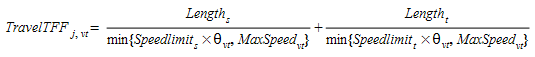
The difference with the travel time in free flow conditions regardless of vehicle type, is that the average maximum speed of vehicle type vt, MaxSpeed~vt~ and the speed limit acceptance of vehicle type vt, θvt. is used to assess the travel time. The latter parameter ( θ > 0) is the ‘level of goodness’ of the drivers or the degree of acceptance of speed limits. A value of θ~vt~ ≥ 1 means that the vehicle adopts a maximum speed greater than the speed limit for the section, while θ~vt~ ≤ 1 means that the vehicle will use a lower speed limit.

The difference with the travel time in free flow conditions regardless of vehicle type, is that the average maximum speed of vehicle type vt, MaxSpeed~vt~ and the speed limit acceptance of vehicle type vt, θvt. is used to assess the travel time. The latter parameter ( θ > 0) is the ‘level of goodness’ of the drivers or the degree of acceptance of speed limits. A value of θ~vt~ ≥ 1 means that the vehicle adopts a maximum speed greater than the speed limit for the section, while θ~vt~ < 1 means that the vehicle will use a lower speed limit.

• Length~j~* is the length of link j in kilometers.
• φ is a user-defined attractiveness weight parameter that allows the user to control the influence of the link attractiveness on the cost in relation to the travel time.
• CL~max~ is the theoretically estimated maximum link attractiveness in the network.
• τ is a user-defined cost weight parameter that allows the user to control the influence of the user-defined cost on the total cost.
• UserDefCost~s~ is the user defined cost of the link j, that is the sum of the section user defined cost plus the turn user defined cost.

Dynamic Cost Function

The Dynamic Cost Function is used when there is simulated travel time data available. Therefore it can only be used when the simulation has already started and data has been gathered. The default current cost for each section is the mean travel time, in seconds, for all simulated vehicles that have crossed the link during the last data gathering time period.

As for the Initial Cost Function, there are also two types of default dynamic cost function. The first, DynCost~j~ is applied to all vehicle types, which means they have the same cost. The second,DynCost~j,vt~, differentiates between vehicle types, which means that there is a dynamic cost function per vehicle type. Which one to use is determined by the presence of reserved lanes in the network.

The default Dynamic Cost for link j common to all vehicle types, DynCost~j~, is a function of the mean travel time, in seconds, for all simulated vehicles that have crossed the link during the last statistics gathering period (TravelTime~j~). The travel time for link j includes the travel time of section s plus the travel time for turn movement t.

There might be situations in which no vehicles have crossed a link, in which case no information about travel time is available. The following algorithm is then applied to calculate EstimatedTravelTime~j~:

if (Flow > 0) then
    EstimatedTravelTime = TravelTime
else
    if (there is any vehicle stopped) then
        EstimatedTravelTime = AvgTimeInSection
    else
        EstimatedTravelTime = AverageSectionTravelTime
    endif
endif
EstimatedTravelTime = Maximum(EstimatedTravelTime, TravelFF)

According to this algorithm, when some vehicles have crossed link j during the last data gathering period (Flow~j~ > 0), the estimated travel time (EstimatedTravelTime~j~) is taken as the simulated mean travel time. If no vehicle has crossed link j, we must distinguish between a totally congested link and an empty link. In the first case, the travel time is calculated as the average waiting time for vehicles waiting in front of the queue in section s (AvgTimeInSection~s~). In the second case, the travel time is taken as the section travel time, which means considering all the turn movements that have as origin section s (AverageSectionTravelTime~s~). All calculated travel times have to be greater than or equal to the travel time of the link in free-flow conditions.

Finally, the Dynamic cost of link j, DynCost~j~, taking into account the penalty for the turn t that belongs to the link and its attractiveness, CL~j~ is calculated as:

where

• EstimatedTravelTime~j~ is the estimated travel time of the link j calculated using the previous algorithm.
• Length~j~is the length of link j in kilometers.
• φ is a user-defined attractiveness weight parameter that allows the user to control the influence that the link attractiveness has in the cost in relation with the travel time.
• CL~max~ is the theoretically estimated maximum link attractiveness in the network.
• τ is a user-defined cost weight parameter that allows the user to control the influence of the user-defined cost on the total cost.
• UserDefCost~s~ is the user defined cost of section s plus the user-defined cost of the turn, which belongs to link j.

The default dynamic cost for link j and vehicle type vt: DynCost~j,vt~, is a function of the mean travel time, in seconds, for all simulated vehicles of type vt that have crossed the link during the last data gathering period (TravelTime~j,vt~). The travel time for link j includes the travel time of section s plus the travel time for turn movement t.

There might be situations in which no vehicles that belong to vehicle type vt have crossed a link, in which case no information about travel time is available, the following algorithm is then applied to calculate EstimatedTravelTime~j,vt~:

if (Flow(j,vt) > 0) then
    EstimatedTravelTime(j,vt) = TravelTime(j,vt)
else
    if (there is any vehicle vt stopped) then
        EstimatedTravelTime(j,vt) = AvgTimeIn(s,vt)
    else
        if (link j has reserved lanes of vehicle class cl) then
            if (vt belongs to cl) then
                if (FlowClass(j,cl) > 0) then
                    EstimatedTravelTime(j,vt) = TravelTimeClass(j,cl)
                else
                    if (there is any vehicle belonging to cl stopped) then
                        EstimatedTravelTime(j,vt) = AvgTimeInClass(s,cl)
                    else
                        EstimatedTravelTime(j,vt) = AverageSectionTravelTime(s,cl)
                    endif
                endif
            else
                if (FlowClass(j, not cl) > 0) then
                    EstimatedTravelTime(j,vt) = TravelTimeClass(j,not cl)
                else    
                    if (there is any vehicle not belonging to cl stopped) then
                        EstimatedTravelTime(j,vt) = AvgTimeInClass(s,not cl)
                    else
                        EstimatedTravelTime(j,vt) = AverageSectionTravelTime(s,not cl)
                    endif
                endif
            endif
        else
            if (Flow(v=j) > 0) then
                EstimatedTravelTime(j) = TravelTime(j)
            else
                if (there is any vehicle stopped) then
                    EstimatedTravelTime(j) = AvgTimeInSection(s)
                else
                    EstimatedTravelTime(j) = AverageSectionTravelTime(s)
                endif
            endif
        endif
    endif
endif
EstimatedTravelTime(j, vt) = Maximum(EstimatedTravelTime(j, vt),
TravelFF(j, vt)

According to this algorithm, when a vehicle of type vt has crossed link j during the last data gathering period (Flow~j,vt~ > 0), the current cost is taken as the simulated mean travel time. If no vehicle of type vt has crossed link j, we distinguish between different cases of costs calculated according to the following steps (each step is carried out if no information is available for the preceding step):

• AvgTimeIn~s,vt~ : Average waiting time for first vehicle of vehicle type vt in front of the queue in the section.

• If section s has reserved lanes for vehicle class cl:

  • and vehicle type vt uses the reserved lane:
    • TravelTimeClass~j,cl~: Is the Mean Travel Time of link j aggregating all vehicle types of vehicle class cl.
    • AvgTimeInClass~s,cl~: Is the average waiting time for first vehicle of vehicle class cl in front of the queue in the section s.
    • AverageSectionTravelTime~s,cl~ : Is the average section travel time of all vehicles of vehicle class cl.
  • and vehicle type vt does not use the reserved lanes:
    • TravelTimeClass~j,not\ cl~: Is the Mean Travel Time of link j aggregating all vehicle types not belonging to vehicle class cl.
    • AvgTimeInClass~s,not\ cl~: Is the average waiting time for first vehicle not belonging to vehicle class cl in front of the queue in the section s.
    • AverageSectionTravelTime~s,not\ cl~: Is the average section travel time of all vehicles not belonging to vehicle class cl.

• If section s does not have reserved lanes:

  • TravelTime~j~: Is the Mean Travel Time of link j aggregating all
  • vehicle types.
  • AvgTimeIn~s~: Is the average waiting time for first vehicle in front of
  • the queue in section s.
  • AverageSectionTravelTime~s~: Is the average section travel time for all types.

All calculated travel times have to be greater than or equal to the travel time of the link in free-flow conditions.

Finally, the Dynamic Cost of link j of vehicle type vt: DynCost~j,vt~, taking into account the penalty for the turn t that belongs to the link and its attractiveness CL~j~, is calculated as:

where:

• EstimatedTravelTime~j,vt~ is the estimated travel time of vehicle type vtof link j calculated with the previous algorithm.
• Length~j~ is the length of link j in kilometers.
• φ is a user-defined attractiveness weight parameter that allows the user to control the influence that the link attractiveness has in the cost in relation with the travel time.
• CL~max~ is the theoretically estimated maximum link attractiveness in the network.
• τ is a user-defined cost weight parameter that allows the user to control the influence of the user-defined cost on the total cost.
• UserDefCost~s~ is the User defined cost of link j, that is the sum of the section user defined cost plus the turn user defined cost.

User-defined link cost functions

The default cost functions, described above, are defined in terms of link travel time only and do not explicitly consider other influences, for example toll pricing, historical travel times representing driver’s experience from previous days, combinations of various link numerical attributes as for instance travel times, delay times, length, and attractiveness, etc. Therefore, for each link, a user-defined cost function can be used which includes these attributes. This is created with the Cost Function editor, as described in the Functions section.

The user-defined cost functions can use the most common mathematical functions and operators (+ , -, *, /, ln, log, exp, etc.). The function terms can be defined as parameters, constants, and variables but must correspond to numerical attributes of an object in the model (links, sections, turns, vehicle types, etc.), whose values could be either fixed (i.e. lengths, theoretical capacities, number of lanes, etc.) or change during the simulation (i.e. link flows, average link speeds, average link travel times, etc.).

Two types of user-defined cost functions can be distinguished: Basic cost functions (named Cost Function) and cost functions considering Vehicle Type (named Cost Function with Vehicle Type).

Basic cost functions do not distinguish between vehicle types and therefore cannot make use of variables that have any vehicle type reference. The parameters for this type of function are: S (the section reference of the link) and T (the turn reference of the link). Cost functions considering Vehicle Type can distinguish between vehicle types and consequently can make use of variables derived from the vehicle type . The parameters for this type of function are: S (the section reference of the link), T (the turn reference of the link) and the vehicle type VT reference.

If the user-defined cost function considers vehicle type data associated with any link of the network, the calculation of shortest paths is made per vehicle type, otherwise it is common for all vehicle types.

Route Paths

Shortest Path Algorithm

During the simulation, the shortest paths are calculated at every time interval t (the Route Choice Interval). The shortest path routine is a variation of Dijkstra's label-setting algorithm, Dijkstra (1959), and it provides as a result the shortest path tree for each destination centroid. This provides the shortest path from the start of every section to that destination centroid. As this includes the turning penalties, the cost labels are attached to links rather than to the network nodes.

The shortest path routine is based on link cost functions. Therefore, the costs of all links are evaluated/updated before the paths are computed. At the beginning of the simulation, the initial cost function is evaluated per each link and, during the next time intervals, the dynamic cost function is used.

The shortest path routine generates a shortest path tree for each destination centroid d(SPT~d~,d ∈ D), but there is an extra step that identifies new paths for all OD pair i ∈ I, taking SPT~d~,d ∈ D, and adds to the set of alternatives path K~i~ of OD pair i. From one shortest path tree, there are as many paths SP~con~ as connectors con for the origin centroid.

The generic schema of the Dynamic Traffic Assignment is:

Step 0: Calculate initial shortest path(s) for each OD pair using the defined initial costs.

Step 1: Simulate for a predefined time interval (e.g. 5 minutes) assigning to the available path the fraction of the trips between each OD pair for that time interval according to the selected route choice model and obtain new average link travel times as a result of the simulation.

Step 2: Recalculate shortest path, taking into account the experienced average link travel times.

Step 3: If there are guided vehicles, or variable message signs suggesting a route change, provide the information calculated in 2 to the drivers that are dynamically allowed to update path en route.

Step 4: Go to step 1.

And the algorithm, including the details of shortest path calculation, is as follows:

Step 0: Calculate initial shortest path(s) for each OD pair using the defined initial costs

• Step 0.1:Initialization:
  • Evaluate Initial Cost Function per each link j:
  • for each j ∈ (1... L) :
    • Cost~j~ = InitialCost~j~
• Step 0.2: Apply Shortest Path routine:
  • for each destination centroid d:
    • Calculate Shortest Path Tree SPT~d~ using Cost~j~ j ∈ (1... L)
• Step 0.3: Identify Shortest Path from Shortest Path Tree:
  • for each OD pair i (from origin centroid o to destination d)
    • Add to Path(s) SP~con~ to K~i~

Step 1: Simulate for a predefined time interval Δt assigning to the available path K~i~ the fraction of the trips between each OD pair i for that time interval according to the selected route choice model.

Step 2: Recalculate shortest path, taking into account the average link travel times from the simulation.

• Step 2.1: Update Link Cost Functions:
  • Evaluate Dynamic Cost Function per each link j:
  • for each j ∈ (1... L) : Cost~j~ = DynamicCost~j~
• Step 2.2: Apply Shortest Path routine:
  • for each destination centroid d:
  • Calculate Shortest Path Tree SPT~d~ using Cost~j~ j ∈ (1... L*)
• Step 2.3: Identify Shortest Path from Shortest Path Tree:
  • for each O-D pair i (from origin o to destination d)
    • Add to Path(s) SP~con~ to K~i~

Step 3: If there are guided vehicles, or variable message signs suggesting a route change, provide the information calculated in 2 to the drivers that are dynamically allowed to update path en route.

Step 4: Go to step 1.

Initial K-Shortest Paths

At the beginning of the simulation, using the initial cost function, a shortest path tree is calculated for each destination centroid, all vehicles are therefore assigned to the same alternative during the first interval. To consider more than one alternative, as a way of anticipating the assignment process, k shortest path trees can be calculated at the beginning of the simulation using the K-initials shortest path function.

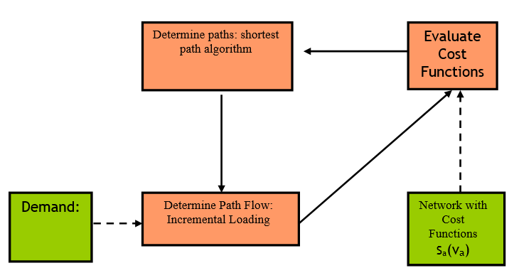
The algorithm executes an incremental static assignment, calculating at every iteration a new shortest path until the number of shortest path trees available reaches the parameter Initial K-Shortest Paths and loading at each iteration the 100/K % of the demand. The figure above shows the generic scheme of the algorithm that, iteratively:

• Evaluates the cost function in each link. In the first iteration the cost function is the initial cost function (travel time in free-flow conditions by default) and in the following iterations the cost function is the K-initials shortest paths cost function.
• Calculates a new shortest path.
• Determines the path flow using an incremental loading procedure, described below and updates the flow in each link.

The components of this algorithm are:

• The Shortest Path Algorithm which computes the shortest path and corresponds to a variation of Dijkstra’s label setting algorithm.

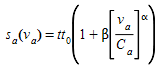
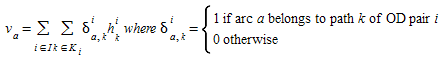
• The Link Cost Function which is a function of link a, s~a~(v~a~), is function of the flow in link a, v~a~

  

• The Incremental Loading Algorithm which assigns the demand. The path flow rates in the feasible region satisfy the conservation of flow and non-negativity constraint (where the traffic demand of OD pair i is denoted by g~i~ and the path flow assigned to path k of OD pair i is denoted by h^i^~k~). That is:

  

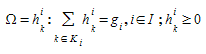
  For each OD pair i ∈ I and path h^i^~k~, evaluate the path flow assigned to the path h^i^~k~ k ∈ K~i~ at iteration n :

  

  

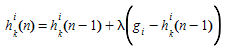
  where

K Shortest path

The algorithm to calculate the k-shortest path can be stated as follows (n is the iteration index and k is the shortest path index):

Step 0: Initialization: n=0 and k=1

• Compute the k-th shortest path based on the free-flow travel times (using the Initial Cost function)
• For each O-D pair i ∈ I,
  • assign h^i^~k~(n)=g~i~ / InitialK-SP

Step 1: Compute the flow v~a~ for each link a:

• Evaluate the cost function of each arc a (s~a~(v~a~)).

  

Step 2: k= k +1, n = n +1.

• Compute the k-th shortest path based cost function of each arc a (s~a~(v~a~)).

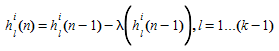
  Incremental Loading: For each O-D pair i ∈ I, evaluate:

  

  

  where

Step 3: If k is equal to total number of shortest path InitialK-SP

• then STOP Otherwise, return Step 1

K-Initials Shortest Path Cost Function

The K-initials shortest path cost function is used at the beginning of the simulation when no simulated data has yet been gathered to calculate the k-initials shortest paths representing a volume delay function. In this case, the cost of each link is calculated as a function of the assigned volume.

There are two types of default K-initials shortest path cost function. For the first type, IniKCost~j~ the vehicle type is not taken into account, that is, all vehicle types have the same K-initial cost. For the second type, IniKCost~j,vt~, the vehicle type is considered, which means that there is a K-initials cost function per vehicle type.

If the user-defined penalty for turn t that belongs to the link is taken into account, the K-initials cost of link j, IniKCost~j~ is calculated as follows:

where

• SectionVDF~j~ is the estimated delay of section s in link j in seconds considering the assigned flow:

  

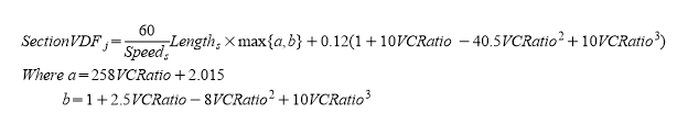
  where Length~s~ is the length, Speed~s~ is the speed of section s, which belongs to link j, in km and VCRatio is the assigned volume of link j divided by the attractiveness of link j.

• TurningPenalty~j~ is the penalty of turn t in link j in seconds considering the turn speed as follows:

  

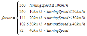
  TurningLength is the length of the turn in km.

• τ is a user-defined cost weight parameter that allows the user to control the influence of the user-defined cost on the cost.

• UserDefCost~s~is the User-defined cost of section s, which belongs to link j.

The K-initials cost of link j per vehicle type vt, IniKCost~j,vt~,is calculated as the K-initials cost without considering vehicle type except in the case where the turn is not allowed for vt that the cost will be infinite to forbid vehicles go through it.

Path Selection

Path selection, which is based on discrete route choice models or on a user-defined assignment, is used to estimate the path flow rates. Path selection models the driver’s decision of which path to take from a set of alternatives, connecting one origin to one destination. This decision process is made when a vehicle enters the system (Initial Assignment) and also during its trip, when new alternatives are available (En-Route Path Assignment Update).

Given a finite set of alternative paths, path selection calculates the probability of taking each available path and then the driver’s decision is mode by randomly selecting a path according to the probabilities assigned to each alternative. This process corresponds to Step 1 in the generic algorithm of Dynamic Assignment and in combination leads to the following algorithm:

Step 0: Calculate initial shortest path(s) for each OD pair using the defined initial costs

• Step 0.1:Initialization: Evaluate Initial Cost Function per each link j:

  • for each j ∈ 1... L Cost~j~ = InitialCost~j~

• Step 0.2: Apply Shortest Path routine:

  • for each destination centroid d: Calculate Shortest Path Tree SPT~d~ using Cost~j~ j ∈ 1... L

• Step 0.3: Identify Shortest Path from Shortest Path Tree:

  • for each OD pair i (from origin centroid o to destination d)
  • Add to Path(s) SP~con~ to K~i~

Step 1: Simulate for a predefined time interval Δt assigning to the available path K~i~ the fraction of the trips between each OD pair i for that time interval according to the selected route choice model.

• Step 1.1:Assignment of path probabilities:
  • for each O-D pair i:
  • Calculate P~k~using the Route Choice Model,where k ∈ K~i~
• Step 1.2:Simulate for a predefined time interval Δt, generating the fraction of the vehicles between each OD pair i for that time interval, selecting randomly the path according to probabilities P~k ,~k ∈ K~i~

Step 2: Recalculate shortest path, taking into account the experiment average link travel times.

• Step 2.1: Update Link Cost Functions:
  • Evaluate Dynamic Cost Function per each link j:
  • for each j ∈ 1... L
    • Cost~j~ = DynamicCost~j~
• Step 2.2: Apply Shortest Path routine:
  • for each destination centroid d:
    • Calculate Shortest Path Tree SPT~d~ using Cost~j~ j ∈ 1... L
• Step 2.3: Identify Shortest Path from Shortest Path Tree:
  • for each OD pair i (from origin centroid o to destination d)
    • Add to Path(s) SP~con~ to K~i~

Step 3: If there are vehicles which accept updating its path en route, or variable message signs which suggest path updates through traffic management actions; provide the information calculated in step 2 to the drivers that are dynamically allowed to update path en route.

Step 4: Go to step 1.

The candidate paths can be of three different types (explained in the Path Definition section): OD Routes (ODR), Path Assignment Result (PAR) and Calculated Shortest Paths, which can be calculated using the Initial Cost Function Initial Shortest Paths (ISP) or calculated using the Dynamic Cost Function, Dynamic Shortest Paths (DSP).

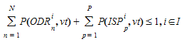
A vehicle of vehicle type vt traveling from OD pair i, can choose one path according to the user-defined assignment or as a result of a Route Choice model from the set of alternative paths K~i~:

• N OD Routes: ODR~n~^i^ n=1..N
• M Path from an Assignment results: PAR~m~^i^ m=1..M
• P Initial Shortest Paths: ISP~p~^i^ , p=1..M
• Q Timely Updated Shortest Paths: DSP~q~^i^, q=1..Q

User-defined Selection

The user-defined selection determines the probability of use for OD routes and for paths assignment result.

For each OD route, the user determines the probability of usage, distinguishing per vehicle type (defined “Path Assignment” folder in OD matrix definition). The user defines the probability of use of each OD route and the probability of use of the initial shortest path:

P(ODR~n~^i^, vt) : Probability of use ODR~n~^i^ by a vehicle type vt

P(ISP~p~^i^, vt) : Probability of use ISP~p~^i^ by a vehicle type vt

Satisfying the condition:

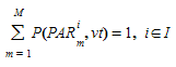
Applying either a static traffic assignment or a dynamic traffic assignment based on Dynamic User Equilibrium experiment, the result is a Path Assignment result, which is a set of paths (PAR~m~^i^) and a percentage of use for each one:

P(PAR~m~^i^, vt) : Probability of use PAR~m~^i^ by a vehicle type vt

Satisfying the condition:

Route Choice Models

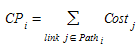
At any time during the simulation, there will be a finite set of alternative paths for each OD pair. The emulation of the driver’s decision of selecting from one of the available paths, that is to assign a trip to a path, is done with a Route Choice model. The Route Choice models are usually based on discrete choice theory that determines the probability for choosing an alternative from a finite set of alternatives as a function of its utility. From transportation point of view, the most common value associated with a trip is the travel time or travel cost, which represents a disutility. Therefore, Route Choice models should be formulated in terms of this negative utility. The most common concept of path cost assumes that it is additive, so the cost of path I, CP~i~, is computed as the sum of the costs of the links Cost~j~ (explained above) composing the path:

The default Route Choice models available are: Proportional, Multinomial Logit, and C-Logit, but others can also be defined using the function editor.

Fixed Routes Mode Vs. Variable Route Mode

In the Fixed Routes Mode, shortest path trees are calculated from every section to every destination centroid at the beginning of the simulation. Then, during the simulation, vehicles are generated at origin centroids and assigned to the shortest route to their destination centroid. There is no need for a Route Choice Model as there are no alternative routes. No new routes are recalculated during simulation. Therefore, all vehicles always follow the shortest path and no decisions about changing to another path can be made during the trip.

Depending on the type of cost function used for the initial shortest path calculations, there are two alternative fixed route models. These are the Fixed using Travel Time in Free Flow Conditions (formerly identified as Fixed-Distance) and the Fixed using Travel Time during Warm-up Period (formerly identified as Fixed-Time) models.

In the Fixed using Travel Time in Free Flow Conditions Model, the paths are calculated at the beginning of a simulation, taking the initial cost as the cost of each arc, whether a warm-up period is defined or not. If there is a warm-up period, no new shortest paths are calculated when it ends, and therefore the same shortest path trees are used during the stationary simulation period. The next figure illustrates when the shortest paths (SP) are calculated in a time diagram of the simulation period.

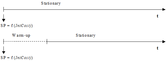
The Fixed using Travel Time during Warm-up Period Model works in a similar way to the Fixed using Travel Time in Free Flow Conditions Model, except when a Warm-up period is defined. In this case, initial paths are calculated at the beginning of the Warm-up in the same way using the Initial Costs. However, when the Warm-up period is over, and the stationary simulation starts, new initial paths are calculated using the Cost Function (calculated using the statistical data gathered during the simulation warm-up) for link costs. The next figure illustrates the shortest paths (SP) calculations in a time diagram of the simulation period.

In the Fixed using Travel Time in Free Flow Conditions Model, the cost does not take into account network congestion, only the length of the paths and the allowed speed. It is labeled Fixed using Travel Time in Free Flow Conditions Model to denote that the cost is mainly based on the distances, together with the speed limits and the attractiveness, but not on the traffic conditions at any given time. In the Fixed using Travel Time during Warm-up Period Model the cost is influenced by the traffic conditions and therefore it represents the travel time more accurately.

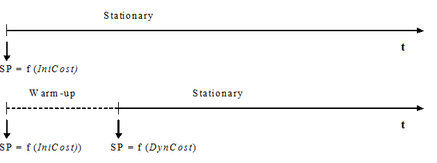
In the variable routes mode, the simulation process includes: an initial calculation of shortest routes going from every section to every destination, a shortest route component that calculates periodically the new shortest routes according to the new travel times provided by the simulator, and a route selection model.

At the beginning of the simulation, shortest path trees are calculated from every section to each destination centroid, taking as link costs the initial cost function, as in the previous case. If a Warm-up period is defined, these paths are calculated at the beginning of the Warm-up. If not, they are calculated at the beginning of the stationary simulation period.

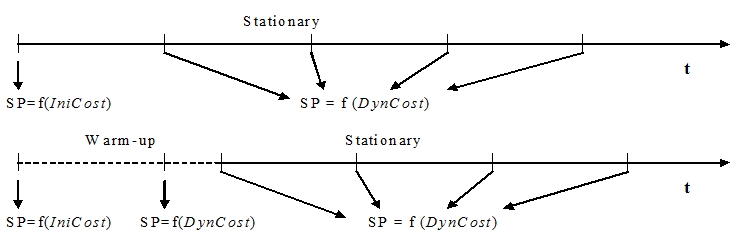
During simulation, new paths are recalculated in every time interval, taking as link costs the simulated travel times obtained for each arc during the last interval. This is the cost function explained above. The next figure illustrates when the shortest paths (SP) are calculated over the simulation period and what cost functions are used.

The time interval for recalculation of paths is defined in the Experiment Editor. It is assumed that vehicles only choose between the best K path trees. These K paths are the pats calculated in the previous intervals plus the OD Routes defined in the OD matrices. Only n OD Routes will be added to the set of possible paths. This n parameter is defined in the Experiment Editor.

Currently four choice models are implemented. They are used either when assigning the initial path for a vehicle at the beginning of its trip or when having to decide whether to change path en route within dynamic modeling. These models are the Binomial, Proportional, the Multinomial Logit and the C-Logit models. Other Route Choice Models can defined using the Cost Function Editor.

Dynamic Assignment

When an OD matrix has been loaded into an Aimsun model, the simulation experiment must be route based. Before running the model,which type of Route Choice Model to use and its parameters is set in the DTA tab of the experiment editor.

There are four route choice models which require parameters to control the route behavior for each OD pair these are:

• Binomial: probability.
• Proportional: alpha factor.
• Logit: scale factor.
• C-logit: scale factor, beta, and gamma.

The parameters are set in the Parameters subtab of the Dynamic Traffic Assignment tab in the Experiment Editor

Binomial Model

A Binomial (k-1, p) distribution is used to find the probability of selecting each path. Parameter k is the number of available paths and p is the “success” probability. This model does not consider the travel costs in the decision process, but only the time at which the path was calculated. Selecting a small p will mean that oldest paths will be more likely to be used, while selecting high values of p, will cause the more recent paths to be taken more frequently.

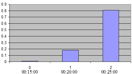
For example, if the goal is to keep three alternative paths and have the newest paths be used more often, then define k=3 and p=0.9. Then the possible values for X = Binomial (2, 0.9) are X = 0,1,2 which are respectively associated with the last three paths calculated. Assume the interval time to recalculate the shortest paths is 5 minutes and the current simulation time is 25:30. In this case, the last three paths calculated have been calculated at times 15:00, 20:00 and 25:00, thus correspondingly X = 0 to 15:00, X = 1 to 20:00 and X = 2 to 25:00. Then, the probability of selecting the oldest path is P(X=0) = 0.01, the probability of selecting the second path is P(X=1) = 0.18 and the probability of selecting the newest path is P(X=2) = 0.81 (The next figure illustrates the binomial model with k=3 and p=0.9).

The ‘success’ probability p can be defined via the Experiment Editor Route Choice parameters Tab when the Binomial model is chosen.

Proportional

The choice probability P~k~ of a given alternative path k , where k ∈ K~i~, can be expressed as:

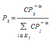
where CP~i~.is the cost of path i.

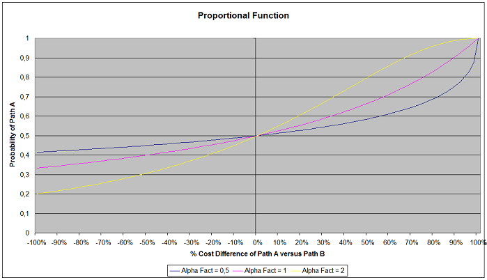
When α =1, then the probability is inversely proportional to path costs. The next figure shows the role of the alpha factor, as a function of the different path costs.The alpha factor can consequently be used to adjust the effect that small changes in the travel times might have on the driver’s decisions.

Multinomial Logit

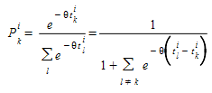
The choice probability P~k~ of a given alternative path k, where k ∈ K~i~, can be expressed as a function of the difference between the measured utilities of that path and all other alternative paths:

or its equivalent expression:

where V~i~ is the perceived utility for alternative path i and θ is a shape or scale factor and V~i~ = -CP~i~/3600 (function V~i~ is the negative of the cost of path i, measured in hours).

We assume that the utility of path k between OD pair i is given by:

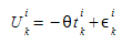
Where:

• θ is a shape or scale factor parameter
• t~k~^i^ is the expected travel time on path k of OD pair i
• ε~k~^i^ is a random term

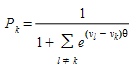
The underlying modeling hypothesis is that random terms ε~k~^i^ are independent identically distributed GUMBEL variates. Under these conditions, the probability of choosing path k amongst all alternative routes of OD pair i is given by the logistic distribution:

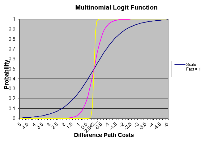
The scale factor θ plays a two-fold role, making the decision based on differences between utilities independent of measurement units and influencing the standard error of the distribution of expected travel times:

where if:

• θ < 1 high perception of the variance, in other words a trend toward utilizing many alternative routes.
• θ > 1 alternative choices are concentrated in very few routes.

For example, given four alternative path with expected travel time (cost path) of T1=12 minutes, T~2~=15 minutes, T~3~=16 minutes and T~4~=18 minutes, the corresponding probabilities when θ = 1 are: P~1~=0.93407, P~2~=0.04650, P~3~=0.01710 and P~4~=0.00231, whereas if θ = 0.5 the probabilities are: P~1~=0.71009, P~2~=0.15844, P~3~=0.09610 and P~4~=0.03535.

The next figure depicts the role of the scale factor, as a function of the difference between path costs:

C Logit

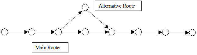
The Logit models exhibit a tendency toward route oscillations in the routes used, with the corresponding instability resulting in a flip-flop process. According to our experience, there are two main reasons for this behavior. The properties of the Logit function and the inability of the Logit function to distinguish between two alternative routes when there is a high degree of overlapping. Some researchers Cascetta (2001) have reported these drawbacks.

The instability of the routes used can be substantially improved when the network topology allows for alternative paths with little or no overlapping at all, changing the shape factor and recomputing the path very frequently. However, in large networks where many alternative paths between origin and destinations exist and some of them exhibit a certain degree of overlapping (see next figure), the use of the Logit function might still exhibit some weaknesses.

To avoid this drawback the C-Logit model, (Cascetta 2001), has been implemented. In the C-Logit model, which is, in fact, a variation of the Logit model, the choice probability P~k~, of each alternative path k ∈ K~i~ of available paths connecting an OD pair, is expressed as:

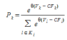
where V~i~ is the perceived utility for alternative path i (expressed in hours) and θ is the scale factor, as in the case of the Logit model.

The term CF~k~, denoted as ‘commonality factor’ of path k, is directly proportional to the degree of overlapping of path k with other alternative paths. Thus, highly overlapped paths have a larger CF factor and therefore smaller utility with respect to similar paths. CF~k~ is calculated as follows:

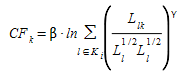
where L~lk~ is the cost of links common to paths l and k, while L~l~ and L~k~ are the cost of paths l and k respectively (expressed in hours). Depending on the two factor parameters β and γ, a greater or lesser weighting is given to the ‘commonality factor’. Larger values of β means that the overlapping factor has greater importance with respect to the utility Vi. The factor γ is a positive parameter, usually taken in the range [0, 2], whose influence is smaller than β and which has the opposite effect on the choice.

As a rule of thumb, it is suggested factor β is in the range [t~min~, t~max~], with t~min~ = Min~k∈Ki~ [CP~k~] and t~max~ = Max~k∈Ki~ [CP~k~]. Then β will become a scaling factor for CF~k~, which translates it into an order of magnitude similar to V~k~ in the formula V~k~ - C~k~ used for the exponential. And thus, when using larger values for β, it is possible that the ‘commonality factor’, CF~k,~will have a greater influence on the choice probability than the utility (i.e. the travel time) itself, thus giving higher probability of choosing non-overlapped longer paths than heavy overlapped shortest paths. Note the commonality factor is not applied to the best alternative.

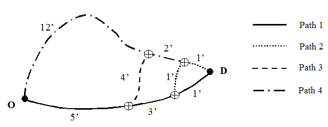
The following is an example to illustrate the use of C-Logit, comparing it with the Multinomial Logit. The figure shows an example network with four alternative paths between origin O and destination D. The table represents the resulting choice probabilities of both models.

Travel Times Path 1 Path 2 Path 3 Path 4 ------------- ------ ------- ------- ------- seconds 540 600 720 900
minutes 9 10 12 15
hours 0.15 0.16 0.2 0.25

Overlapping (llk) v

l / k 1 2 3 4
------ -------- ------ ------- ------- 1 0.1500 0.1333 0.0833 0.0000
2 0.1333 0.1667 0.1000 0.0167
3 0.0833 0.1000 0.2000 0.0500
4 0.0000 0.0167 0.0500 0.2500
CFk 0.126519 0.135793 0.121803 0.039960

with Beta = 0.15 and Gamma = 1.

Example of LOGIT

Scale Factor P(1) P(2) P(3) P(4)
--------------- --------- ------ ------ ------------- 1 0.260448 0.256143 0.247746 0.235663
10 0.354498 0.300076 0.215014 0.130412
20 0.450502 0.322799 0.165730 0.060969
30 0.532071 0.322717 0.118721 0.026490
40 0.599856 0.307976 0.081182 0.010987
50 0.656417 0.285278 0.053882 0.004423
60 0.704153 0.259044 0.035058 0.001745
100 0.836359 0.157968 0.005635 0.000038
500 0.999760 0.000240 1.3885E-11 1.9283E-22
1000 1 0 0 0
2000 1 0 0 0
3600 1 0 0 0

Example of C-LOGIT

Scale Factor P(1) P(2) P(3) P(4) ---------------- --------- -------- --------- --------- 1 0.280102 0.240493 0.235886 0.243519 10 0.608338 0.132440 0.109147 0.150074 20 0.876849 0.041560 0.028227 0.053364 30 0.969831 0.010007 0.005601 0.014561 40 0.993062 0.002231 0.001029 0.003678 50 0.998414 0.000488 0.000186 0.000912 60 0.999635 0.000106 0.000033 0.000225 100 0.999999 0.000000 0.000000 0.000001 500 1.000000 0.000000 0.000000 0.000000 1000 1.000000 0.000000 0.000000 0.000000 2000 1.000000 0.000000 0.000000 0.000000 3600 1.000000 0.000000 0.000000 0.000000 4000 1.000000 0.000000 0.000000 0.000000

The scale factor parameter, θ, and the commonality factor parameters, β and γ, can be defined via the Route Choice parameters tab when the C-Logit model is selected.

User-defined Route Choice Model

As an alternative to the default Route Choice Models, User-defined Route Choice Models can be used. This is done using the Cost Function Editor. Refer to the Functions section for more information on defining the cost functions.

Determine the finite set of paths in the decision process

The path selection based on discrete route choice models, estimates the path flow rates of a finite set of alternative paths K~i~, connecting the i-th OD pair and this set of alternative paths is updated considering the shortest path trees calculated every interval of the Dynamic Traffic Assignment.

At time interval t, the shortest path algorithm is applied and it generates the shortest path tree SPT~d~(t) per each destination centroid d∈D. Then for each OD pair i∈I (with origin centroid o and destination centroid d) and taking SPT~d~(t) it generates one path SP~con~(t) for each connector con linked to the origin centroid.

The process to determine the finite set of paths to be used in the decision process receives as a parameter the “MaxNumberToKeep (which represents the maximum number of most recent shortest paths to consider), MaxNumberOfRoutes (which represents the maximum number of different paths) and UseBestEntrance of centroid origin.

The algorithm is as follows:

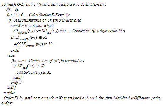
When the origin centroid option Use Origin Percentages is selected, each connector is considered independently to the others, assigning to each connector the percentage of the demand generated by the centroid and applying the route choice model per each connector.

Initial Assignment

The Initial Assignment is the path selection process when a vehicle enters the system. It corresponds to Step 1 in the generic algorithm of Dynamic Traffic Assignment.

A vehicle of vehicle type vt traveling from OD pair i, can choose one path according to the user-defined assignment or as a result of a Route Choice model from the set of alternative paths K~i~:

• N OD Routes: ODR~n~^i^ n=1..N
• M Path from an Assignment results: PAR~m~^i^ m=1..M
• P Initial Shortest Paths: ISP~p~^i^ , p=1..M
• Q Timely Updated Shortest Paths: DSP~q~^i^, q=1..Q

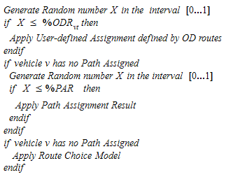
The Initial assignment is determined by the percentage of use the OD routes (%ODR~vt~) and the percentage of use of a Path Assignment Result (%PAR~vt~) (can be determined per vehicle type and set in Route Choice parameters):

Defining the following functions:

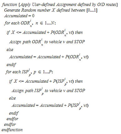
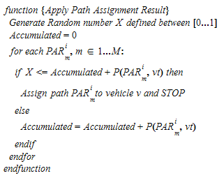
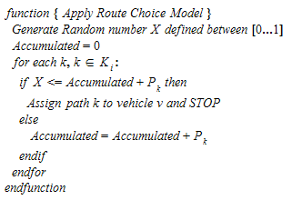
Then the algorithm of Initial Assignment is defined as:

As an example:

Assume that for one vehicle type vt:
 %ODR = 40%
 %PAR = 70%
Assume there are two OD Routes defined with the %use:
 P(ODR1) = 10%
 P(ODR2) = 50%
Assume there are two paths from a Assignment result with %use
 P(PAR1) = 30%
 P(PAR2) = 70%
Assume there are three calculated paths and the Route Choice model assigns %use:
 P(DSP1) = 30%
 P(DSP2) = 20%
 P(DSP3) = 50%

Then the final percentages of vehicle type vt assigned to each path are:
 ODR1 = 40% * 10%
 ODR2 = 40% * 50%
The vehicles not assigned to one ODR then:
 PAR1 = [(1- 40%) + (40% *(1-10%-50%)] * 70% * 30%
 PAR2 = [(1- 40%) + (40% *(1-10%-50%)] * 70% * 70%
The vehicles not assigned to either one ODR or one PAR then:
 DSP1 = [(1- 40%)+ (40% *(1-10%-50%)] * (1-70%) *30%
 DSP2 = [(1- 40%)+ (40% *(1-10%-50%)] * (1-70%) * 20%
 DSP3 = [(1- 40%)+ (40% *(1-10%-50%)] * (1-70%) *50%

En-Route Path Assignment Update

Vehicles are initially assigned to a path from a set of available paths based on probability. After the initial assignment, which is made at the time of the vehicle’s departure, there is the possibility of making a path reassignment during the trip (En-Route Path Update).

The En-Route Path Assignment Update corresponds to Step 3 in the generic algorithm of Dynamic Traffic Assignment and it is applied when the En-Route Path Update parameter is selected in the Dynamic Traffic Assignment folder in the experiment editor.

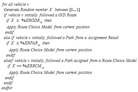
The en-route path assignment update is determined by the en-route path assignment update percentage of vehicles that follow an OD route (%ERODR~vt~), the en-route path assignment update percentage of vehicles that follow a path result of an assignment result (%ERPAR~vt~) and the en-route path assignment update percentage of vehicles that follow a path assigned by the Route Choice model (%ERRCM~vt~) (can be determined per vehicle type and set in the Stochastic Route Choice Parameters tab:

Path Assigned After Virtual Queue

This option can be used to reassign the path for all vehicles that are in a virtual queue. The reassignment is calculated at every route choice time interval.

Entrance/Exit Section decision

When the route choice model is applied to a vehicle on the initial assignment, the first step is to decide the entrance section at which the vehicle will enter the system and the exit section at which it will exit. This decision is made considering the use of percentages on the origin and destination centroid (attribute of centroid). There are 4 different situations:

Origin Centroid considers Percentages / Destination Centroid considers Percentages

The example in the figure below demonstrates the decision process, Here the origin centroid has 3 connections (A, B and C) with 30%, 20% and 50% loading assigned respectively and the destination centroid has 3 exit connections (X, Y and Z) with 40%, 10% and 50%. The only feasible combinations that the connectivity of the network allows are that from connection B, it is possible to reach connection X, Y and Z, while from connection C, it is possible to reach connection Y and Z.

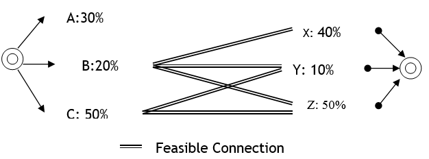
The first step is to decide the entrance section. This process takes into account only the feasible connections available to reach the destination and recalculates the percentages considering the original percentage over the sum of percentages of all feasible connections. In this example, the value for A is 0% (not feasible), B is 20%/70% (70% is the sum of 20% and 50%) and C is 50%/70%. Using these calculated percentages as probabilities, the vehicle chooses the connector i.e., the entrance section, it will use.

After the entrance section is selected, the exit section is chosen. This is done by considering only the feasible connections from the selected entrance section and recalculating the percentages as the original percentage over the sum of percentages of all feasible connections. In this example, if the entrance section chosen uses connection C, then the calculated probability of connection X will be 0% (not feasible from connection C), Y will be 10%/60% (60% is the sum of 10% and 50%) and Z will be 50%/60%. The vehicle then chooses the exit section using these probabilities.

Origin Centroid considers Percentages / Destination Centroid does not consider Percentages

In this case, the entrance section is selected as in the previous case and the exit section depends on the shortest path.

Origin Centroid does not consider Percentages / Destination Centroid considers Percentages

In this case the exit section is selected as in the previous case considering only the feasible connectors from the origin. The entrance section is selected by considering the route choice model.

The Use Best Entrance parameter sets whether the route choice algorithm will take into account, for each origin centroid and for each calculation, only the one shortest path from the entrance with the lowest cost (Use Best Entrance checked) or one shortest path from each entrance section (Use Best Entrance not checked).

Origin Centroid does not consider Percentages / Destination Centroid does not consider Percentages

The entrance section and the exit section are selected by considering the route choice model.

The Use Best Entrance parameter sets whether the route choice algorithm will take into account, for each origin centroid and for each calculation, only the one shortest path from the entrance with the lowest cost (Use Best Entrance checked) or one shortest path from each entrance section (Use Best Entrance not checked).