Time Series
Time series hold observations of a variable made over time. The variable observations can be produced by a simulator (speed on a road, vehicle’s number of stops…); they can come from real world data as detection measures or be calculated as an aggregation of several values (level of service for nodes).
Aimsun Next offers a collection of tools to visualize, compare, and print this data. It is possible to show one or more time series of a single object a vehicle, a section… and also to show several (related) time series of multiple objects.
Time Series for a Single Object
When the variables of an object have values appropriate for time series view, they are displayed in the object editor. The editor will contain a new tab called Time Series. Simulation objects, such as sections, detectors, and simulated vehicles have time dependent data such as speed and distance attached to the object. Replications and Averages listed on the Project window will also have this tab after being simulated/calculated to display data derived from the simulation such as aggregated delay or number of vehicles. In this tab, up to ten time series from the object can be visualized at the same time.
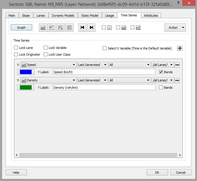
Variables
The Variables/ Graph button toggles the display mode. In Variables mode the object attributes to be displayed are selected; press the plus button to add a new variable or the minus button by each variable to delete it. For each variable the result can be filtered, here the filters for speed and flow are by lane and by user class. The source of the data; a replication, an average or the Last Generated is also specified here for each variable. It is therefore possible to show in the time series plot for the object the results from different experiments on the same graph by taking data from different sources.
The Lock check buttons lock all the variables in the time series to be the same. i.e. Lock Lane forces all displayed variable to use the same lane filter. Lock Originator forces all displayed variables to use the same data source, etc.
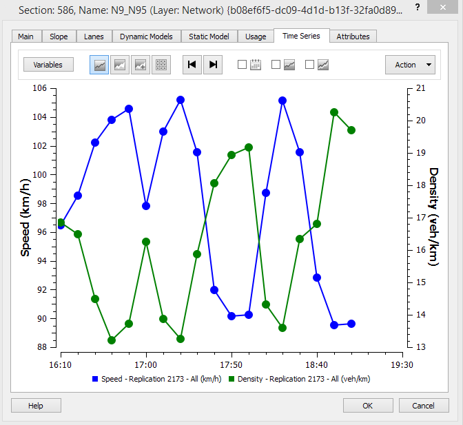
Up to two variables with different units can be shown, either using the left and right scale of the graph (here speed and density are used) or using the X and Y axis, replacing Time on the X axis. The time series data for the variables must share the same simulation interval and a common time period (although time series might have different lengths).
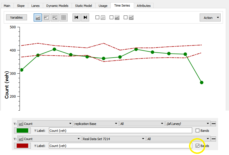
The Bands option shows the minimum and maximum bands of a variable - for example if a Real Data Set has the value and the range ( i.e the maximum and minimum) of that value then this can also be displayed on the time series.
Graphs
This tab displays the data in three ways:
- Graph: This option plots the selected time series.
- Area: This option plots the selected time series as a filled area. There are two possibilities, to show the data as it is, or to sum the time series to the next one before drawing it, accumulating values.
- Table: This option shows the numeric values of the selected time series.
The Use Date must be activated when the time series date in the time series to be compared must to be used. In this case, only time series matching in time and date can be simultaneously plotted. When this option is not checked, only the time value in the time series will need to match.
When the data is represented in Graph mode, the limits of the graph can be adjusted (selecting the desired option in the Adjust limits menu, inside the Action menu) either taking into account the current object values only or all the object's values for the time series. Taking into account all the objects' values is useful when several objects must be compared, as the different graphs will be in the same scale.
If the Deviation option is checked, then for time series that consist of mean values, the deviation will be shown for each value in both the table and the graph
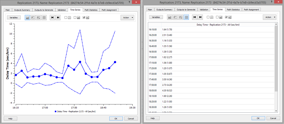
If the Bands option is checked, then the bands will be included in the graph as shown below. Note the real data set here contained the minimum and maximum count values, The simulated value lies mostly in that range
Time Series for Multiple Objects
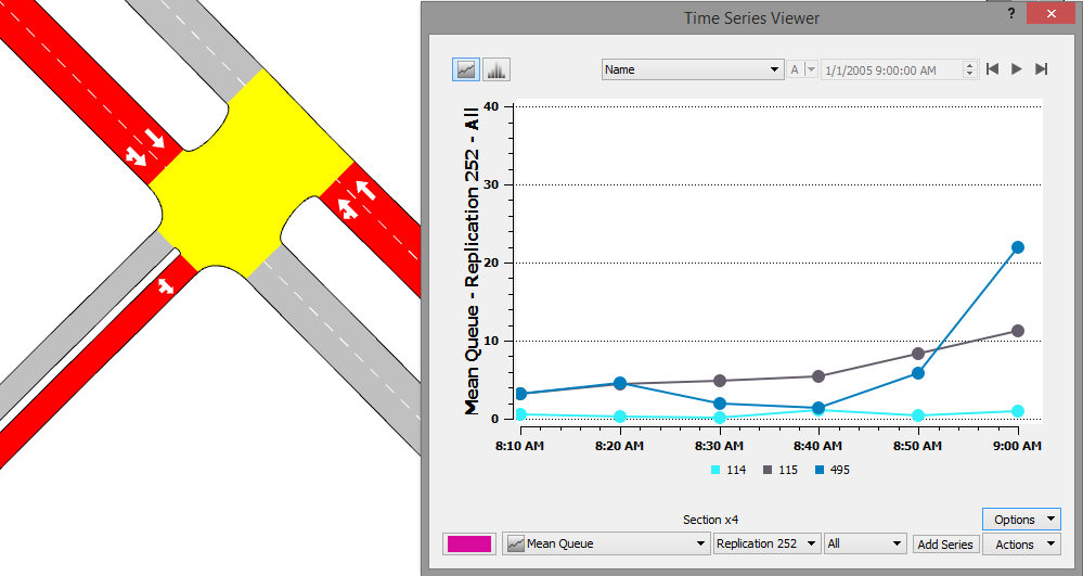
Time series data from several objects can be shown using the Time Series Viewer available from the Data Analysis: Time Series Viewer menu.
There are two ways to plot the time series:
- Temporal graph: Displays the whole time series as a curve using the time as the abscissa.
- Bar Chart: Displays the values of the selected time series at a specific time in a bar chart. The time is defined using the widget in the top-right corner of the Time Series Viewer where a specific time can be selected or the series can be played through the simulation time.
The label drop-down selects the label used to identify objects ( ID, name ...) and the average (A) drop-down selects the average data measure which is shown if the time series is aggregated.
Adding Time Series
With the dialog open, press on any object on a 2D View to select it. Replications and Averages listed on the Project window can also be selected. The available time series from the object will appear in the Time Series combo box. Choose the desired time series and press the Add button. Repeat the selection operation to choose more objects and more time series.
When the first time series has been chosen, only time series with units which are compatible with this first time series can be added. The Time Series combo box will only show the compatible variables for the second and subsequently selected objects.
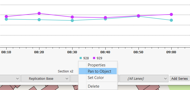
Managing Individual Time series
Clicking on the time series label in the Time Series plot brings up a menu to; show the properties dialog of the object, pan to the object in the view window, set the color of the series using a color picker dialog or delete this series from the plot.
Actions
The actions menu contains:
- Copy Data: see Copying Data to the Clipboard.
- Copy Graph (Snapshot): see Copying Data to the Clipboard.
- Set Scale... : opens a dialog to define the Min and Max of the ordinate axis of the graph.
- User Defined Scale : adjust the ordinate axis to the Min and Max defined with the "Set Scale..." action.
- Auto Scale: adjust the ordinate axis to the values of the displayed Time Series of the displayed objects.
- Auto Scale (All Objects): same as "Auto Scale", but considering all the objects of the network.
- Clear: clears the graph of all its Time Series.
- Clear and Unselect: same as "Clear" and also unselecting all selected objects in the view.
Options
The options menu contains:
- Use Date: take the date information of the Time Series into account (uncheck this option to compare two Time Series that occur at the same time but at different days).
- Show Value Labels: display the value of each point of the Time Series as a text label on the graph.
- Draw Scale Marks: display horizontal scale marks in the background of the graph.
- Smooth Curve: display the Time Series as smoothed curves (instead of the default straight-lines).
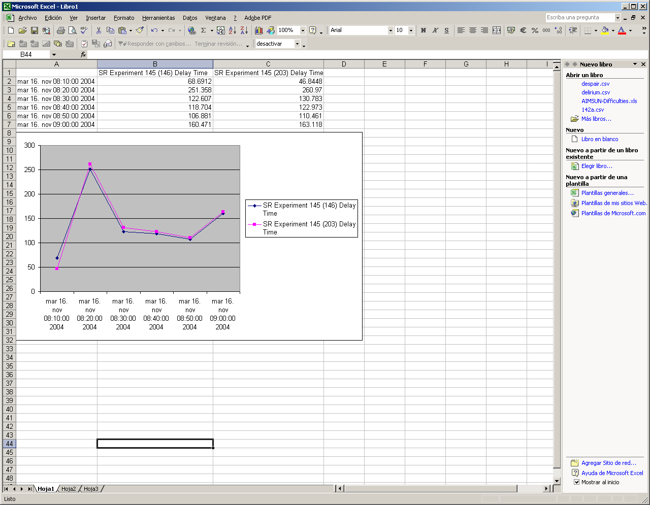
Copying Data to the Clipboard
When Aimsun Next shows a time series, either in an object editor or in the Time Series Viewer, the displayed data can be copied to the system clipboard. Activate the Copy command by pressing the Action button then selecting Copy Data (to copy the data in tabular format) or Snapshot (to copy a snapshot of the time series) or using its shortcut (CONTROL+C). The data can then be pasted to an application such as Excel or Gnumeric.