Modeling Vehicle Movement

The process of moving vehicles in a microsimulation model is described in the following sections, listed below.

• Vehicle Entry
• Car Following
• Two-Lane Car Following
• Adaptive Cruise Control (ACC) and Cooperative Adaptive Cruise Control (CACC) car-following
• Lane Choice
• Lane Change
• Lane Change Gap Acceptance
• Ramp Merge
• Gap Acceptance
• Two-Way Overtaking
• Modeling Acceleration in Microscopic Simulation
• Driver Parameters
• Parameters

Vehicle Entry

Arrivals

The OD Matrix or the Traffic State specified in the Traffic Demand object describes how many vehicles will enter the simulation network at each connector from each centroid. The Arrivals algorithms control when those vehicles arrive in the simulation and the headways between them. The arrivals algorithms are Exponential, Uniform, Normal, Constant, External, and ASAP and are documented in the Arrival Algorithm section.

Entry

The calculation to determine whether there is enough space for a vehicle to enter the network uses the parameters from the entrance section, the parameters of the last vehicle (the leader) that entered the entrance section and the parameters of the vehicle that is trying to enter.

Entrance section parameters:

• the Speed Limit (MaxSectionSpeed).

Leading vehicle parameters:

• the current position (Pos) of the vehicle.
• the current speed (Speed) of the vehicle.
• the normal deceleration (MaxDecel) for the vehicle type.
• the length (L) for the vehicle type.
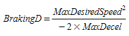
• the braking distance of the leader defined as the distance necessary to stop it by applying the maximum deceleration:

The parameters of the vehicle trying to enter:

• the Mean Maximum Desired Speed (MaxSpeed).
• the Mean Speed Limit Acceptance (θ).
• the Mean Maximum Deceleration (MaxDecel).
• The maximum desired speed on the entrance section defined as:

• the minimum following distance between this vehicle and the leader
• the braking distance of the entering vehicle defined as as the distance necessary to stop it by applying the Normal Deceleration:

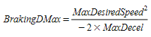
The possible space to enter (PH: Possible Headway) is then defined as:

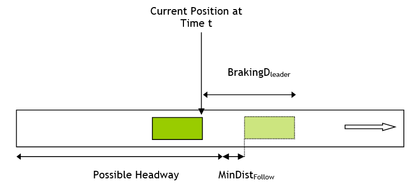
and the space require (MinDistEnter) is the braking distance for the entering vehicle. Therefore to enter safely the logic is:

if (PH >= MinDistEnter) then 
    The vehicle has enough space
Else
    The vehicle does not have enough space
Endif

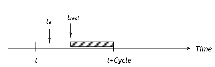
To place the vehicle in the network, the entrance time and position are derived as follows.

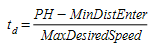
The time t~d~ needed to travel distance d is:

Therefore, the entrance time t~real~ is defined by:

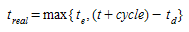
where:

• t~e~ is the theoretical entrance time
• t is the simulation time
• cycle is the simulation step

When the entrance time is known, then the entrance position is then defined by:

Virtual Entrance Queues

When a vehicle entrance is scheduled by the Arrival Algorithm, but there is not enough space to enter, then the vehicle is placed in a virtual queue for that section. This is shown in the Virtual Queues Tab of the Section Editor. The definition of virtual entrance queues depends on the traffic generation and the arrival algorithm used to introduce vehicles into the simulation.

If the Traffic demand is defined as a Traffic State:

• Traffic generation model- Exponential, Uniform, Normal, and Constant: The virtual entrance queue is defined as a list of vehicle types. The entrance process consists of taking the first element of the list and generating the vehicle. If the size of the list is greater than a set value, then Aimsun Next gives a warning message.

  An example of virtual queue for one entrance section could be
  Car     Car     Bus     Taxi    Car Truck   Car ...
  

• Traffic generation model- ASAP: The virtual entrance queue is defined as a list of elements, where each element represents a vehicle type and the number of vehicles of that type awaiting entry. The entry process takes a randomly selected vehicle from the list preserving the ratio of vehicle types.

  An example of a virtual queue for one entrance section could be:
      Vehicle Type        Number of Vehicles      
      -------------       ------------
      Car                 10
      Bus                 2
      Taxi                4
      ...                 ...
      Truck               2
  

If the Traffic demand is defined as an OD Matrix

• Traffic generation model- Exponential, Uniform, Normal, and Constant: The virtual entrance queue is defined as a list of elements, where each element represents the vehicle type identifier, its origin, and its destination. The entry process takes the first element of the list and generates the vehicle. If the size of the list is greater than a set value, then Aimsun Next gives a warning message.

  An example of a virtual queue for one entrance section could be:
      -------     -------     --------    -------     --------    --------    --------    ------
      Car         Car         Bus         Taxi        Car         Truck       Car         ...
      From 1      From 1      From 4      From 1      From 1      From 1      From 1      ...
      To 2        To 3        To 2        To 2        To 2        To 2        To 3        ...
  

• Traffic generation model- ASAP: There is no virtual entrance queue as vehicles are generated in the simulation as soon as there is a space for them.

Behavioral models

During their journey through the network, vehicles are updated according to vehicle behavior models: “Car-Following” and “Lane-Changing”. Drivers tend to travel at their desired speed in each section but the environment (i.e. the preceding vehicle, adjacent vehicles, traffic signals, signs, blockages, etc.) will condition their behavior.

The simulation time is split into small time intervals called simulation cycles or simulation steps (t). This value can be set within the range (0.1 ≤ t ≤ 1.5 seconds). At each simulation cycle, the position and speed of every vehicle in the network is updated according to the following algorithm:

if (necessary to change lanes) then
    Apply Lane-Changing Model
endif
Apply Car-Following Model

Once all vehicles have been updated for the current cycle, vehicles scheduled to arrive during this cycle are introduced into the system and the next vehicle arrival times are generated.

Car-Following Model

First, some terms are defined in traffic flow theory to describe the relative positions of vehicles measured in time and distance.

• Headway: The time between the front bumper of a vehicle and the front bumper of the following vehicle
• Gap: The time between the rear bumper of a vehicle and the front bumper of the following vehicle
• Spacing: The space between the front bumper of a vehicle and the front bumper of the following vehicle
• Clearance: The space between the rear bumper of a vehicle and the front bumper of the following vehicle

These will be used in the following description of vehicle behavior

The car-following model implemented in Aimsun Next is based on the Gipps model (Gipps 1981 and 1986b). It has been developed by including model parameters which are not global but determined by the influence of local parameters depending on the “type of driver” (speed limit acceptance of the vehicle), the geometry of the section (speed limit on the section, speed limits on turns, etc.), the influence of vehicles on adjacent lanes, etc.

It consists of two components, acceleration and deceleration. The first represents the intention of a vehicle to achieve a certain desired speed, while the second reproduces the limitations imposed by the preceding vehicle when trying to drive at the desired speed. This model states that the maximum speed to which a vehicle (n) can accelerate during a time period (t, t+dt) is given by:

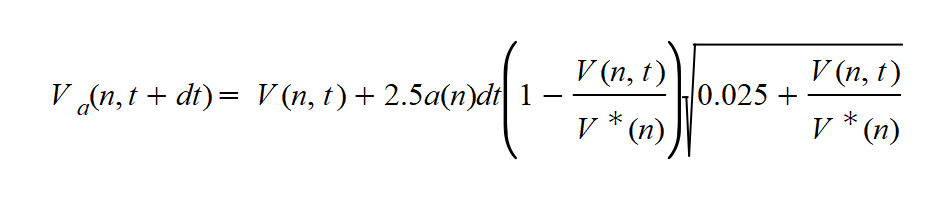
where:

• V~a~(n,t) is the speed of vehicle n at time t;
• V*(n) is the desired speed of the vehicle (n) for current section;
• a(n) is the maximum acceleration for vehicle n;
• dt is the simulation cycle;

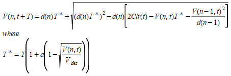
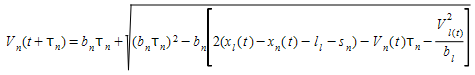
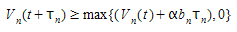
At the same time, the maximum speed that the same vehicle (n) can reach during the same time interval (t, t+dt), according to its own characteristics and the limitations imposed by the presence of the lead vehicle (vehicle n-1) is:

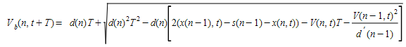
where:

• d(n) (< 0) is the maximum deceleration desired by vehicle n;
• x(n,t) is position of vehicle n at time t;
• x(n-1,t) is position of preceding vehicle (n-1) at time t;
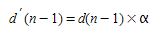
• s(n-1) is the effective length of vehicle (n-1);
• d'(n-1) is an estimation of vehicle (n-1) desired deceleration;
• T is the reaction time.

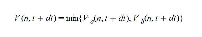
The speed for vehicle n during time interval (t, t+dt) is then the minimum of these two speeds

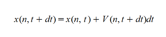
The position of vehicle n in the current lane is then updated using the integration of the speed. Acceleration and deceleration phases are integrated using different methods. The acceleration phase is integrated using the rectangle method corresponding to the following equation:

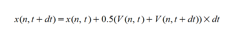
while the deceleration phase integration uses the trapezoid method following this equation:

The estimation of the leader’s deceleration is a function of the Sensitivity Factor parameter α defined per vehicle type. The model is then:

When α is < 1, the vehicle underestimates the deceleration of the leader and as a consequence the vehicle becomes more aggressive, decreasing the gap ahead of it.

When α is greater than 1, the vehicle overestimates the deceleration of the leader and as a consequence the vehicle becomes more careful, increasing the gap ahead of it.

The model also includes the minimum headway between leader and follower as a restriction of the deceleration component. This constraint is applied before updating the position X(n,t+T).

The minimum headway constraint is defined as:

If

then

where:

• x(n,t) is position of vehicle n at time t;
• x(n-1,t) is position of preceding vehicle (n-1) at time t;
• MinHW(n) is the minimum headway of vehicle (n) between it and vehicle (n+1).

Note that the headway is used in this formula. Previously, the gap was used and this has been corrected here.

Modified Model for Congested Highways

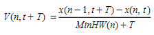
The speed predicted by the Gipps car-following model at high density does not match the speeds observed under congested conditions in highways. A modified model is used to adjust the dependency of the speed as a function of density. This is achieved by changing the dependency of the inter-vehicular distance (Clearance) as a function of speed which is simply linear in the Gipps model.

The equation from Gipps for the clearance between vehicles is:

which is transformed to:

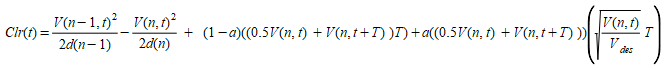
and

At constant speed and maximum deceleration, this simplifies to:

The effect on clearance and flow is shown below.

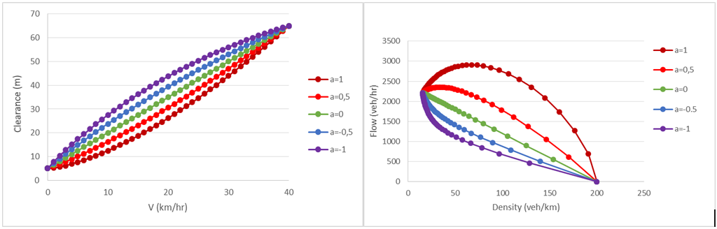
This was tested on a network where the density of traffic was increased to the point where flow breakdown was observed.

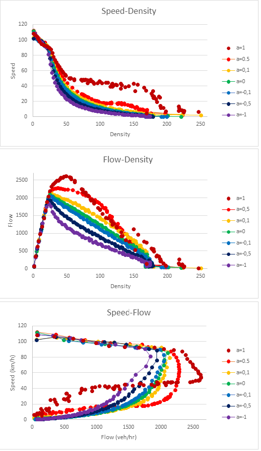
The a parameter range is set by the vehicle type and each car, when generated, is assigned a value for a which it keeps while it is in the simulation. As the effect of a is different in acceleration and deceleration, there is an option to use +a in acceleration and -a in deceleration. Hence, if a is positive, the clearance between vehicles will be larger during acceleration than deceleration for the same speed.

Calculating the speed for a vehicle at a section

The car-following model is such that a leading vehicle, i.e. a vehicle driving freely, without any vehicle affecting its behavior, would try to drive at its maximum desired speed. Three parameters are used to calculate the maximum desired speed of a vehicle while driving on a particular section or turn, two are related to the vehicle and one to the section or turn:

• Maximum desired speed of the vehicle i: v~max~(i)
• Speed limit acceptance of the vehicle i: θ(i)
• Speed limit of the section or turn s: S~limit~(s)

The speed limit for a vehicle ion a section or turn s, is calculated as:

The maximum desired speed of vehicle i on a section or turn s, is calculated as:

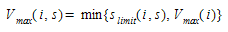
This maximum desired speed V~max~(i,s) is the same as that referred to above, in the Gipps car-following model, as V*(n)

The Two-lane Car-Following Model

The Two-lane Car-Following Model: Absolute

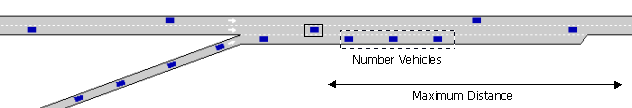
The goal of the two-car lane-following model is to include the influence of the vehicles in adjacent lanes in the car-following model. When a vehicle is driving along a section, the model considers the influence that a specified number of vehicles (Number Vehicles) driving slower in the adjacent right-side lane (or the left-side lane, when driving on the left), might have on the vehicle. The model then determines a new maximum desired speed of a vehicle in this section, which will be used in the car-following model.

The parameters for the Two-Lane Car Following Model are set in the Experiment Editor: Behavior Tab and the correspondence between lanes is either determined by their common section or can be determined through adjacent subpaths as described below.

The model first calculates the mean speed for Number Vehicles driving downstream of the vehicle in the adjacent slower lane (MeanSpeedVehiclesDown). Only vehicles within a certain distance (Maximum Distance) from the current vehicle are taken into account (see Figure below). If less than Number Vehicles are involved, the desired speed of the current vehicle at the section is used to add vehicles to make up Number Vehicles values in order to get a more meaningful average.

There are two cases: 1) the adjacent lane is an on-ramp and 2) the adjacent lane is any other type of lane. Apart from Number Vehicles andMaximum Distance parameters, two more parameters are defined:Maximum Speed Difference and Maximum Speed Difference On-Ramp. Then, the final desired speed of a vehicle at a section is calculated as follows:

if (the adjacent slower lane is an On-ramp) {
    MaximumSpeed = *MeanSpeedVehiclesDown* + *MaximumSpeedDifferenceOnRamp*
} else {
    MaximumSpeed = *MeanSpeedVehiclesDown* + *MaximumSpeedDifference*
}

This procedure ensures that the differences of speeds between two adjacent lanes will be less than or equal to the Maximum Speed Difference or Maximum Speed Difference On-Ramp, respectively.

Note that when either the vehicle's current lane or its adjacent lane are reserved and set to not be considered in the Two-lane Car-following Model, then the model is not applied.

Example

The following example is intended to clarify the influence of the Number of Vehicles parameter. Assume that Number of Vehicles = 4 and Maximum Distance = 100m. This means that a vehicle looks at the first 4 cars in front of it in the adjacent lane that are located in the next 100 meters from its position and takes their average speed. If there are only 2 cars in this 100 meters section, only the speed of these cars are considered, and to get the 4 vehicle average speed, 2 additional 'dummy' cars with free flow speed are included.

For instance, assume that in the next 100 meters there is an on ramp with 1 vehicle stopped and 1 moving at 40 km/h and speed limit of the section is 60 km/h. The average speed considered in two-lane car following would be:

(0 + 40 + 60 + 60)/4 = 40 km/h.

If the maximum speed difference at on-ramps is 50 km/h, it would mean that vehicles in the main lane would accept driving at 50 + 40 = 90 km/h.

If however, there were 4 cars or more stopped in the ramp, the average speed would be 0 km/h and this would mean that vehicles in the main lane would accept driving at 50 + 0 = 50 km/h. If there are moving cars further than 100 meters away, they would not affect the vehicle until it approached them when it would progressively include them in the calculations.

The Two-lane Car-Following Model: Relative

This model assumes that a vehicle driving in a fast lane will reduce speed in the presence of slow vehicles in an adjacent lane to anticipate that a slow vehicle might pull out in front of it.

Considering that the fast vehicles are driving at the speed limit and the slow vehicles at the speed limit minus the speed difference, the model calculates how many of the upcoming slow vehicles in a homogeneous platoon might be assumed by the faster vehicle to not change lane.

The maximum speed of the faster vehicle is then calculated using the usual Car-Following model so as to avoid collision with the next untrusted slow vehicle if it was to change lane.

The safe spacing between the two vehicles is defined as:

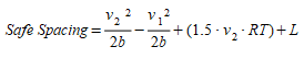
where v~1~ and v~2~ are the speeds of the vehicles, b is the deceleration, RT the reaction time and L the length of the leading vehicle.

Example

For example, if the speed limit of the road is 120 km/h and the speed difference used in the two-lane model is given as 40 km/h:

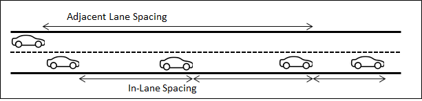
• The safe space required to avoid collision between a vehicle traveling at V~2~=120 km/h and a vehicle traveling at V~1~=80 km/h (speed limit of the road minus the speed difference) is 132.16 meters, where b=4 m/s\^2^, RT=1s and L =5m. This is represented as “Adjacent Lane Spacing” in the image below:

• The in lane spacing between two vehicles of an homogeneous queue (Interpreted as V~1~=V~2~ and using the same deceleration) traveling at V~1~=80 km/h is 38.33 m

• The number of slow vehicles (NSV) corresponding to the safety gap between fast and slow vehicles is NSV= 132.16/38.33=3.44.

If the mean speed in the slower lanes was actually measured to be 60 km/h in the simulation then to calculate the effective speed limit in the faster lane:

• The distance using the safe spacing formula between slow vehicles, taking V~1~= V~2~ = 60 Km/h is 30m
• The safe spacing for the faster vehicles, using the previously calculated NSV is 30*3.44 = 103,42 meters This distance is used to calculated V~2~ using the safe spacing formula between fast and slow vehicles and taking V~1~= 60km/h. V~2~ = 97,86 km/h

This value of v~2~ is then speed limit of the fast lane, modified by the model to take into account the adjacent slower traffic.

The Two-lane Car-Following Model: Adjacent Paths

In some cases, adjacent lanes can be modeled in separate road sections and vehicles will adjust speed to merge when the sections converge but while they are still separate. In this case, the adjacency is determined not by looking across lanes in the same road section, but by looking at across subpaths defined in the adjacent sections.

In this case, if two subpaths start and finish at the same nodes, i.e. they are adjacent lanes modeled as separate sections, then they can be linked in the subpath editor and the same two-lane car-following model, based on distance along the subpath to determine adjacency will be used.

Adaptive Cruise Control (ACC) and Cooperative Adaptive Cruise Control (CACC) car-following

It is possible to use an ACC/CACC module that uses different models to compute the acceleration of a vehicle depending on the cruise controller choices.

Note that although the vehicle type reaction time should stay to the human reaction time value (i.e. 0.8s), the ACC/CACC controller has been implemented to work on autonomous vehicle simulation steps (0.1s). On one side, then, the experiment simulation step in the Reaction Time tab should be changed to 0.1 to see the effects of the ACC/CACC models in the simulation. On the other, the Reaction Time settings should be set to Variable (Different for Each Vehicle Type) so that the vehicles reaction time is not equal to the simulation step.

ACC/CACC Modules

• Speed Regulation mode: a_sv=k₁*(v_f-v_sv)

  where:

  • a_sv: acceleration recommended by the ACC controller to the subject vehicle (m/s2).
  • k₁: gain in the speed difference between the free flow speed and the subject vehicle’s current speed (s⁻¹). It corresponds to the parameter called Speed Gain Free Flow on ACC tab of the vehicle type editor.
  • v_f: free flow speed (m/s).
  • v_sv: current speed of the subject vehicle (m/s).

• ACC Gap Regulation mode: a_sv=k₂(d-t_hw v_sv-L)+k₃(v_l-v_sv )

  where:

  • a_sv: acceleration recommended by the ACC controller to the subject vehicle (m/s2).
  • k₂: gain on position difference between the preceding vehicle and the subject vehicle (s⁻²). It corresponds to the parameter called Distance Gain on the ACC tab of the vehicle type editor.
  • k₃: gain on speed difference between the preceding vehicle and the subject vehicle (s⁻¹). It corresponds to the parameter called Speed Gain Following on ACC tab of the vehicle type editor.
  • d: distance between the subject vehicle’s front bumper and the preceding vehicle’s front bumper (m).
  • t_hw: desired time gap of the ACC controller (s). It corresponds to the distribution called Desired Time Gap on the ACC tab of the vehicle type editor.
  • v_sv: current speed of the subject vehicle (m/s).
  • L: length of the preceding vehicle (m).
  • v_l: current speed of the preceding vehicle (m/s).

• CACC Gap Regulation mode:

  • Acceleration: a_sv(t)=(v_sv(t)-v_sv(t- ∆t))/∆t
  • Current speed: v_sv(t)=v_sv(t- ∆t)+ k_pe_k (t)+k_de^'_k (t)
  • Time gap error: e_k(t)=d(t- ∆t)-t_g* v_sv(t- ∆t)-L
  • Speed error: e^'_k(t)=v_l (t- ∆t)- v_sv(t- ∆t)-t_g* a_sv (t- ∆t)

  where:

  • a_sv: acceleration recommended by the ACC controller to the subject vehicle (m/s2).
  • v_sv: current speed of the subject vehicle (m/s).
  • Δt: time step for each update (s).
  • k_p and k_d: gains for adjusting the time gap between the subject vehicle and preceding vehicle (k_p in s−1 and k_d have no units). k_p corresponds to the parameter called Distance Gain in the CACC tab of the vehicle type editor and k_d corresponds to the parameter called Speed Gain in the CACC tab of the vehicle type editor.
  • e_k: time gap error.
  • t_g: is the constant time gap between the last vehicle of the preceding CACC string and the subject vehicle (s). It corresponds to the parameter called either Time Gap Leader or Time Gap Follower in the CACC tab of the vehicle type editor, depending on the platoon state of the vehicle.
  • L: length of the preceding vehicle.
  • v_l: current speed of the preceding vehicle (m/s).
  • d: distance between the subject vehicle’s front bumper and the preceding vehicle’s front bumper (m).

ACC/CACC Vehicles

Vehicle types can be equipped with either an ACC or a CACC module (or be non-equipped).

Both modules can perform Speed Regulation Mode, which is typically used when no vehicle is ahead of the current vehicle (or if vehicle ahead is too far).

ACC modules use ACC Gap Regulation mode to control the vehicle movement based on the vehicle ahead if any.

CACC modules use CACC Gap Regulation mode instead.

The distribution of non-equipped vehicles, ACC equipped vehicles and CACC equipped vehicles is defined in each vehicle type editor.

Whenever a vehicle is equipped with an ACC or a CACC module, it will only be functional on roads whose road type allows it.

CACC Platooning

The CACC module equipped vehicles can form platoons, which are groups of consecutive connected vehicles that can have smaller time gaps than normal between them. That is due to the fast and reliable exchange of information from one vehicle to the other.

Platooning is done by implementing two variants of Gap Regulation mode: Follower and Leader. Those variants differ in the Time Gap that is used in the formula.

A Follower is a vehicle that belongs to a platoon and it is not the first one of that platoon.

A Leader is any connected vehicle that is not a Follower.

Platoons have a maximum size. If a vehicle is trying to join a platoon that is full, then it will become a leader of its own platoon instead. Refer to the road type editor to specify the CACC vehicles platoon size settings.

ACC/CACC Emergency Take Over

The ACC/CACC model includes the CAMP forward collision warning algorithm as shown on the paper Using Cooperative Adaptive Cruise Control (CACC) to Form High-Performance Vehicle Streams on pages 22 and 23.

This makes the vehicles being able to change from any ACC/CACC driving modes to Disabled if the algorithm shows a potential collision that will not be avoided by the controller.

If, at any point, the car happens to go to manual driving, aka disabled, due to this algorithm then there is a 20s cooldown for them to be able to go into ACC/CACC driving modes again. This represents an average time for a driver to take care of the situation and judge safe enough to get back to automatic driving modes.

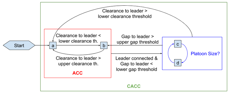
ACC/CACC Decision Chart

Simulation vehicles have a dynamic column that is called ‘Cruise Control Status’ to show which driving mode has been used in the last simulation step. The five possible values are:

a. CC Speed Regulation b. ACC Gap Regulation c. CACC Platoon Leader Gap Regulation d. CACC Platoon Follower Gap Regulation e. Disabled

The decision chart for applying one of the first four modes above is:

Lane Changing Model

The lane-changing model can also be considered as a development of the Gipps lane-changing model (Gipps 1986a and 1986b). Lane change is modeled as a decision process, analyzing the necessity of the lane change (such as for turn maneuvers determined by the route), the desirability of the lane change (to reach the desired speed when the leader vehicle is slower, for example), and the feasibility of the lane change depending on the position of the vehicle in the road network with respect to the lane geometry and adjacent vehicles.

The global parameters that control the lane-changing model are set in the Experiment Editor: Behavior Tab.

The lane-changing model is a decision model that approximates the driver’s behavior as follows at each vehicle update:

• Is it necessary to change lanes? This depends on several factors: the turning options from the current lane, the distance to the next turn and the traffic conditions in the current lane described by speed and queue lengths.

• Is it desirable to change lanes? This depends on whether there will be any improvement in the traffic conditions for the driver as a result of lane changing. This improvement is measured in terms of speed and distance. If the speed in the target lane is faster compared to the current lane, or if the queue is shorter by sufficient margin, then it is desirable to change lanes.

• Is it possible to change lanes? This requires that there is an adequate gap to make the lane change. This calculates both the braking imposed by the future downstream vehicle to the lane-changing vehicle and the braking imposed by the lane-changing vehicle to the future upstream vehicle. If both braking levels are acceptable, then lane changing is possible.

To represent the driver’s behavior in the lane-changing decision process, three different zones are considered, each one corresponding to a different lane-changing motivation.

• Zone 1: The lane-changing decisions are mainly governed by the traffic conditions of the lanes involved. To measure the improvement that the driver will get from changing lanes, several parameters are considered: The desired speed of driver, the speed and distance of current preceding vehicle, speed and distance of future preceding vehicle in the destination lane. The model implemented in this zone is the overtaking maneuver model.

• Zone 2: This is the intermediate zone. Vehicles driving in the "wrong" lane (i.e. lanes where the desired turn movement cannot be made) tend to get closer to the correct side of the road from which the turn is allowed. Vehicles looking for a gap try to adapt their speed to find gaps located either downstream or adjacent to them.

• Zone 3: Vehicles are urgently trying to reach their valid lane, looking for gaps upstream and reducing speed if necessary, even coming to a complete stop in order to make the lane change possible.

The lane changing of each vehicle i at section s has five aspects:

• Lane Changing zone distance calculation
• Target Lanes calculation
• Vehicle behavior considering the target lanes
• Gap Acceptance model for Lane Changing
• Target Gap and Cooperation

Lane-Changing zone distance calculation

Lane-changing zones are delimited by two parameters, the Look-Ahead and the Critical Look-Ahead. Look-ahead is the upstream distance to the point where the vehicle is aware of its target lanes (start of lane-changing zone 2) and the critical look-ahead is the upstream distance to the start of lane-changing zone 3.

These parameters are defined in distance (meters or feet), by default, or time (seconds), depending on the user preferences. When these parameters are defined in time, the conversion to physical distance is calculated as:

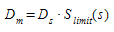
where:

• D~m~: Distance in meters
• D~t~ : Distance in seconds
• S~limit~(s): Speed limit of the section s.

The perception of the Look-Ahead and the Critical Look-Ahead for each vehicle is varied using the vehicle's Minimum and Maximum Look-Ahead Factors. For instance, if a look-ahead is defined as 200 meters, the Minimum Look-Ahead Factor is 0.9 and the Maximum Look-Ahead Factor is 1.2, then the perception of the distance will be from 180 (calculated as 0.9 x 200) to 240 (calculated as 1.2 x 200) meters. All vehicles select their distance from the range 180-240 using a uniform random distribution.

Target Lanes calculation

The lane-changing process starts by calculating the valid target lanes. The output of this process is a set of valid lanes for zone 3 and a set of valid lanes for zone 2.

Vehicle behavior considering the target lanes

The strategy is for every vehicle try to reach the set of target lanes defined by zone 2 and 3 and the vehicle behavior is as follows:

• If the vehicle's current lane is not within the subset of valid lanes determined by Zone 3, the vehicle's behavior is determined by Zone 3.

• If the vehicle's current lane is within the subset of valid lanes determined by Zone 3 but outside of the subset of valid lanes determined by Zone 2, the vehicle's behavior is determined by Zone 2.

• If the vehicle's current lane is within the subsets of valid lanes of both Zone 3 and 2, the vehicle's behavior is determined by Zone 1.

When the current lane of a vehicle is in a valid lane determined by zone 2 and 3, in general the behavior is modeled as if it was in zone 1, i.e. overtaking maneuvers can be initiated. There is an exception when a vehicle's leader is affected by an obstacle (turn movement, incident, lane closure, etc.) that is closer than the vehicle's own obstacle, then the evaluation to overtake the leader includes using a lane that can be outside of the subset of lanes given by Zone 2.

Gap Acceptance model for Lane Changing

The gap acceptance model is consistent with the car-following model, in order to avoid artificial break down situations:

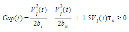
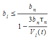
The Gipps car-following model is stable i.e. it does not require decelerations above the maximum desired deceleration αb~n~ where b~n~ is an estimation of the vehicle leader desired deceleration.

This is achieved when:

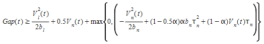
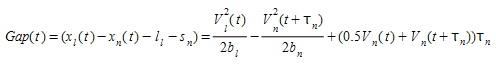
The Gipps car-following model avoids crashes when the Gap remains positive all over the deceleration process. This gives an additional constraint:

This condition must be fulfilled to apply the Gipps car-following model with a new leader when a vehicle changes lane (i.e. selection of possible leader and gap acceptance).

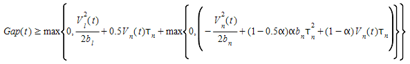
Furthermore, applying this constrain at the end of the deceleration process i.e. when

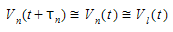
yields:

if the vehicle changes lane, the speed and position of the vehicles at time t+dt is evaluated:

• For the vehicles that are already updated, current speed and position is used.
• For the others, the speed and position assuming that the vehicle changes lane at time t+dt is evaluated.

The gap is acceptable if the physical quantities at time t+dt fulfils the three following requirements:

• the gaps are positive
• the computed speeds are positive,
• the decelerations imposed are smaller than α MaxDesiredDecel

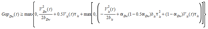
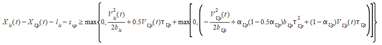
Using the previous equations this can be achieved with one condition at time t that need to be fulfilled for both the upstream and downstream gaps.

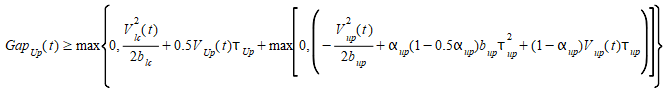
and

The acceptance of the gap in the lane-changing model can be modified by defining the following parameters in the Section Editor: Dynamic Models Tab:

• Aggressiveness: This parameter allows vehicles to enter shorter gaps without forcing the rear vehicle to brake, followed by a relaxation process to gradually recover the stability of the car-following models. The aggressiveness % controls the sensitivity of a vehicle to the deceleration of the leader, determining how short can these gaps be. That is, if aggressiveness is set to 100% (which should not be used, it's the most extreme case) this means zero sensitivity, and the new allowed gap (at all speed situations) would be that needed at a stop situation (as if the vehicle was parking). An aggressiveness 0%, the full gap is used as described above, with no change in sensitivity. All intermediate values will make the gap shorter according to the aggressiveness % and also to the current speed of the leader. Aggressiveness applies to all lane-changing maneuvers that are not cooperative. This parameter can be set for a Road Type or can be adjusted by Vehicle Type.
• Imprudent Lane Changing: This option determines whether vehicles can enter gaps that do not ensure car-following stability. The vehicle changing lane, or its follower, might need to brake up to twice their maximum deceleration. Only vehicles where the vehicle type also has the 'Imprudent lane changing' activated will accept those gaps.

Target Gap and Cooperation

To change lane, the target lane is searched for an adequate gap. The upstream vehicle of the gap must and be able to follow the vehicle that is looking for a gap using the crash free car-following model or be willing to cooperate. The subject vehicle intending to change lane will then progressively adapt to the speed of the downstream vehicle using the two-leaders car-following model with a negative gap if needed. When choosing an adjacent or backward gap, the vehicle intending to change lane will always have a speed that is lower than the one imposed by its current leader. To avoid this penalty, the lane-changing vehicle can instead choose a forward gap if it is able to overtake the downstream vehicle before the forthcoming obstacle. Selecting a forward gap will however not cause it to exceed the Gipps car-following speed imposed by its current leader.

The percentage of upstream vehicles that cooperate in the lane-changing model is defined for each section or vehicle type using the Lane Changing Cooperation parameter in the Road Type Editor or the Vehicle Type Editor. Note that upstream vehicles will only cooperate with requesting vehicles being in Zones 2 and 3; that is, vehicles for which the lane change is compulsory.

The order of evaluation of gaps in each zone is:

• Zone 1
  • 1^st^ Adjacent gap
• Zone 2
  • 1^st^ Forward gap
  • 2^nd^ Adjacent gap
• Zone 3
  • 1^st^ Adjacent gap
  • 2^nd^ Backward gap

Forward Gap Evaluation:

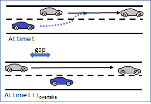
In a forward gap evaluation, the vehicle which plans to change lane assesses a gap in the adjacent lane, ahead of its current position, which requires it to overtake the downstream vehicle in that lane. First, assuming that both the downstream and preceding vehicles maintain their current behavior, the time required to overtake that downstream vehicle is estimated (t~overtake~)

Given the estimated position of the subject vehicle and of the one that will be upstream of it at that time, the critical gap between the two is evaluated and, if that gap is acceptable, the forward gap is selected as target.

The figure below shows the subject vehicle's desired forward gap at time t and the situation at time (t + t~overtake~) when it assesses the gap between it and the vehicle that will be upstream of it at that time. Additionally, the vehicle that will be upstream of the subject, if it cooperates, will then modify its car following from single car following (solid line) with its original leader to apply the two-leaders car-following model (dashed lines) which includes the subject vehicle.

The lane change will be made in a future simulation step if the selected forward gap becomes an adjacent gap that is still acceptable.

The forward gap is scanned only in Zone 2.

Adjacent Gap Evaluation

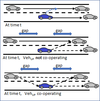
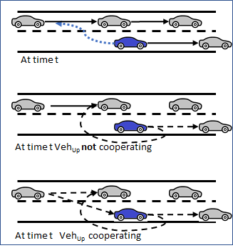
In an adjacent gap evaluation, the subject vehicle which plans to change lane is situated between two vehicles in its target lane and must assess the gaps adjacent to it between both the upstream vehicle (Veh~Up~) and downstream vehicle (-Veh~Dn~) This is done using the Gipps car-following algorithm.

The figure below shows the relationships between the vehicles in an adjacent gap evaluation. At time t, the subject vehicle and Veh~Up~ are using single car following in their respective lanes (solid lines). If both the gaps are acceptable, or the upstream vehicle is willing to cooperate, the adjacent gap is selected and the subject vehicle applies the two-leaders car-following model as shown by the dashed lines. The upstream vehicle either applies the two-leaders car-following model when the gap is selected, if it cooperates, or when the lane-changing maneuver starts, if it does not cooperate.

The adjacent gap is scanned in all zones.

When an adjacent gap is selected, the subject vehicle starts making a lane-changing maneuver when both the gap with Veh~Up~ and the gap with Veh~Dn~ are acceptable, i.e. in the simulation step after the one when the adjacent gap was selected, if the gaps were already acceptable, or when the cooperation of Veh~Up~ has made its gap acceptable.

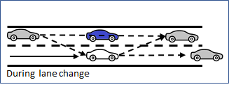
In the figure below, the blue vehicle is the subject. As it makes its lane change, its simulation representation is instantly moved into the new lane but leaves a shadow vehicle in the lane it has just left for the duration of the lane change, which depends on the speed. This provides a vehicle to follow in both lanes for the time during which the subject vehicle spans two lanes.

Backward Gap Evaluation

In a backward gap evaluation, the vehicle which plans to change lane assesses a gap in the adjacent lane, behind its current position, which requires it to reduce its speed until it falls behind a vehicle upstream in that lane. The future follower is selected by taking the closest upstream vehicle in the target lane that would be able to undertake car following with the subject vehicle. The subject vehicle applies the two-leaders car-following model with the current leader of the future follower. If the future follower cooperates, it also applies the two-leaders car-following model with the subject vehicle.

The backward gap is scanned in zone 3.

Two Leaders Car Following

This model is applied when a vehicle is adapting its speed to a second leader. The possible situations are:

• If both leaders are downstream and further away than the critical gap, the vehicle follows the most restrictive leader.
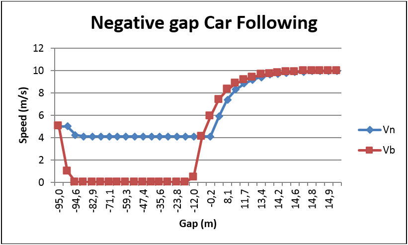
• If one of the leaders is upstream (as in a backward gap assessment) or closer than the critical gap, the deceleration derived by Gipps imposes a sharply decreasing speed down to zero. To avoid this behavior, we constrain the deceleration speed of the follower with:

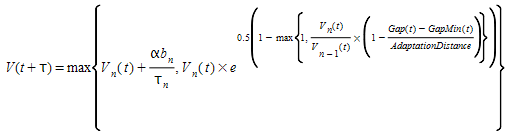
This ensures the speed continuity when the upstream leader passes the vehicle. The Adaptation Distance specifies the point at which this should occur. In the comparison below, the Gipps default implementation is presented in red and the negative gap implementation in blue.

Overtaking Maneuver

An overtaking maneuver takes place in Zone 1 when the vehicle is in its set of valid lanes and changes lane to pass another vehicle. In order to promote or discourage overtaking, there are two parameters:

• Overtake Speed Threshold is the percentage of the desired speed of a vehicle below which the vehicle might decide to overtake. This means that whenever a vehicle is constrained to drive slower than Overtake Speed Threshold % of its desired speed, it will try to overtake. The default value is 90%.

• Lane Recovery Speed Threshold is the percentage of the desired speed of a vehicle above which a vehicle will decide to get back into the adjacent slower lane. The default value is 95%.

Therefore, if a vehicle with a desired speed of 100kph was to follow a vehicle at a speed < 90kph, it would try to overtake. Subsequently, when it achieved a speed > 95kph, it would return to its original lane

It is recommended that the Lane Recovery Speed Threshold value is greater than Overtake Speed Threshold, otherwise some overtaking maneuvers might be aborted as they start. Similarly, if these values are set too small, vehicles will not initiate an overtaking maneuver unless the speed gap is very large and would return to the slower lane too soon.

Note that the sensitivity to these parameters is low.

These two parameters can be edited from the Tables Window for a Dynamic Experiment, from the attributes of a experiment or can be set by vehicle type to override the default experiment parameters.

Return to Lane after Overtake

The tendency to move back to the slower lane after overtaking is determined by the road type, the specific road section, and by the Staying in Overtaking Lane parameter for a vehicle type.

If the road section allows for Return to Inside lane After Overtaking , either set by the road type or modified for the specific road section. Then, after every lane change maneuver, a new value for the Keep Fast Lane Boolean attribute for the vehicle is generated based on the Staying in Overtaking Lane percentage for the vehicle type. If this value is false, then the Lane Recovery Speed Threshold is ignored and the vehicle will remain in the lane it used to overtake.

Determine the side of the maneuver

The road side determines the overtaking maneuver according:

• When a vehicle attempts to overtake another vehicle it will try to do so using the adjacent left lane when driving on the right side, or the adjacent right lane when driving on the left.
• When a vehicle is driving fast enough and wants to move back to the slower lane, it will try to go to the rightmost lane when driving on the right and to the leftmost lane when driving on the left.
• In presence of optional reserved lanes HOV Lane: A vehicle entering a section in which one or more lane is optionally reserved for its vehicle type will consider the closest reserved lane, even if it is not adjacent to its current lane, as an alternative to improve its traffic conditions. If the traffic conditions are better on the reserved lane, the vehicle will try to reach it doing a multiple lane change if needed but without receiving cooperation from other vehicles.

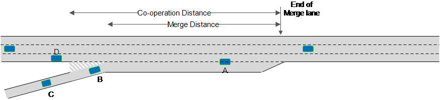
On-Ramp Model

The parameters that control the On Ramp Lane Changing Model are set in the Section Editor: Dynamic Models Tab.

The lane-changing model applied at on-ramps is the same cooperative model as for normal lane changes with three additional controls:

• First vehicle on is first vehicle off: If toggled on, only the first vehicle on the ramp can change lane to move off it, if toggled off, all vehicles on the ramp might try to merge.

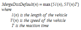
• Merging Distance: The merging distance controls where vehicles start to merge onto the main carriageway. Its default value for vehicle n is 5 times the maximum of the length of the vehicle or 5 times the distance traveled in 1 reaction time. This allows the vehicle to start its merge before it is required to slow at the end of the ramp:

  

• Cooperation Distance: The distance from the end of the ramp where a vehicle can start to receive co-operation from vehicles on the main carriageway to make its lane change.

The difference between these two distances simulates the separation zone at a ramp merge where vehicles on the ramp are visible to the main carriageway but can not yet merge.

In the diagram below:

• Vehicle A is merging onto the main carriageway as it is within the Merge Distance
• Vehicle B is not yet within the Merge Distance and will not move off the ramp but it is within the Co-operation Distance and can expect vehicle D to allow it to make the lane change once it is within the merge distance.
• Vehicle C is not yet within the Co-operation Distance, will not be visible to vehicle D and cannot yet expect any co-operation.
• Vehicle D is aware of A and B, but not C.

Gap-Acceptance Model: Yield Behavior

The parameters that control the Gap Acceptance Model are set in the Road Type Editor : Turn Parameters Tab but the defaults supplied by the road type can be overwritten for each turn using the turn editor in the Node Editor: Turn Editor: Dynamic Models Tab. Each vehicle type can then provide a range of Safety Margin Factor values as multipliers for the safety margin thus affecting the behavior by vehicle type and, within each type, by vehicle too.

Several vehicle parameters also influence the behavior of the gap-acceptance model: turn speed, acceleration rate, desired speed, speed limit acceptance. These are set in the Vehicle Type Editor: Dynamic Models Tab and Microscopic Tab.

A Gap-Acceptance model is used to model yield behavior. This model determines whether a vehicle approaching an intersection can or cannot cross depending on the nearby vehicles with higher priority at the junction. This model takes into account the distance of vehicles to the hypothetical collision point, their speeds and their acceleration rates. It then determines the time needed by the vehicles to clear the intersection and produces a decision that also includes the level of risk of each driver.

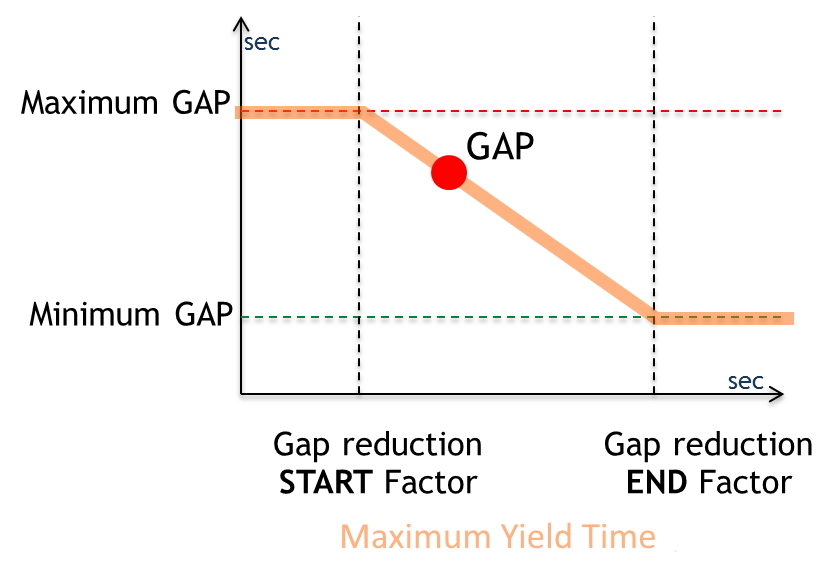
The gap required to make the maneuver is determined by the time spent waiting for a gap to appear in the opposing flows. The initial value is MaximumGap; the final value is MinimumGap. After waiting for GapReductionStartTime * MaximumGap seconds, the gap is progressively reduced, reaching the minimum gap value after GapReductionEndTime * MaximumGap seconds.

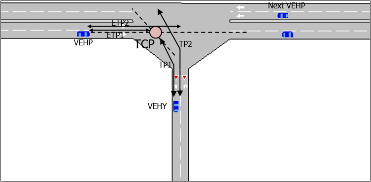
The following algorithm is applied in order to determine whether a vehicle approaching a Yield sign can cross or not. The locations and vehicles are shown in the figure below:

Given a vehicle (VEHY) approaching a Yield junction,

• Obtain the closest higher priority vehicle (VEHP)
• Determine the Theoretical Collision Point (TCP)
• Calculate time (TP1) needed by VEHY to reach TCP
• Calculate estimated time (ETP1) needed by VEHP to reach TCP
• Calculate time (TP2) needed by VEHY to cross TCP
• Calculate estimated time (ETP2) needed by VEHP to clear the junction
• If TP2 (plus the safety margin controlled by the Gap equation presented above) is less than ETP1, vehicle VEHY has enough time to cross; therefore it will accelerate and cross
• Else, if ETP2 (plus a safety margin) is less than TP1, vehicle VEHP will have already crossed TCP when VEHY reaches it, then search for the next closest vehicle with a higher priority, it becomes VEHP and go to step 2
• Else, vehicle VEHY must yield, decelerating and stopping if necessary.

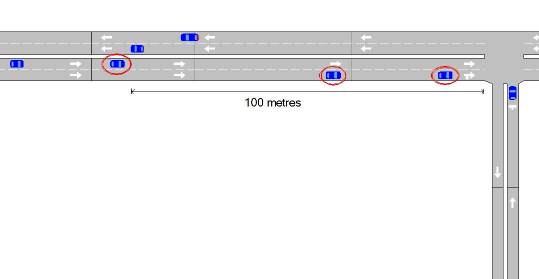
Only higher priority vehicles that are within sections that are within or partially within the visibility distance of the main stream (e.g. 100 meters) of the node will be considered by the lower priority vehicle, as shown by the circled vehicles in figure below.

Two-way Overtaking Model

The Two-way Overtaking Model simulates the overtaking maneuvers on two-lane, two-way rural roads. This model covers the desirability evaluation, the decision, and the execution process and relies on parameters defined in the Experiment Editor: Behavior Tab, the Vehicle Type Editor: Microscopic Tab, and the Section Editor: Dynamic Models Tab.

Network Requirements

Two way overtaking requires that the opposing sections are linked as Mirror sections. This is documented in the Section Editor.

Model Description

The possibility to overtake is considered for the vehicles that are in queue. Each vehicle that cannot reach its desired speed due to downstream traffic conditions is considered to be in queue. The queue leaders are identified as the vehicles triggering the queues, i.e. the vehicle going at its desired speed.

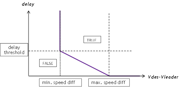
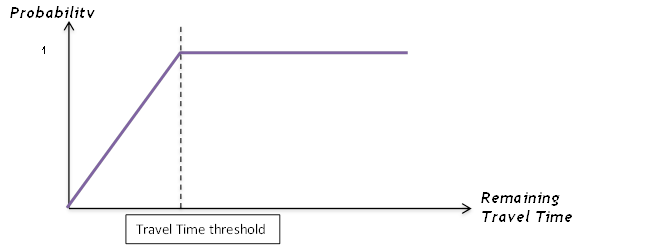
For each vehicle in the queue, the desire to overtake is evaluated based on five characteristics: their rank in the queue, the delay induced by the queue, the speed difference between their desired speed and the actual speed of their immediate leader, and their remaining travel time. The desirability function is defined by parameters defined for the Experiment:

• Delay time threshold
• Minimum speed difference threshold
• Maximum speed difference threshold
• Maximum rank
• Remaining travel time threshold
• Number of simultaneous overtakes allowed
• Delay between simultaneous overtakes
• Sensitivity factor to reduce car following
• Overtaking speed enhancement factor
• Speed difference threshold for enhanced overtaking speed
• Speed difference threshold to overtake with solid line

Two parameters are defined for the section:

• Visibility distance
• Visibility factor

One vehicle parameter is defined:

• Safety margin for the overtaking maneuver

These parameters define the following desirability curves presented in the following figures:

If the vehicle's decision is to overtake, it applies car following with a reduced safety gap using the Car-following distance reduction factor parameter and evaluates the feasibility of the overtaking maneuver.

The decision to initiate the overtake includes verifying that no solid line forbids changing toward the overtaking lane. In the case the vehicle to about overtake is currently been overtaken by other vehicles, it takes into account whether multiple overtaking is allowed, following the number of simultaneous overtaking maneuvers allowed, and whether the delay between simultaneous overtaking, is respected.

If allowed, the overtaking feasibility is evaluated. If the speed difference between the desired speed and the actual speed of the immediate leader is smaller than the speed difference threshold for overtaking speed acceptance, the vehicle will use an enhanced desired speed for overtaking specified by the overtaking speed enhancement factor.

The duration of the overtaking maneuver is calculated assuming the vehicle maintains a constant acceleration until it reaches its desired speed after which it maintains a constant speed. The time to collision with the closest oncoming vehicle is also calculated assuming this also keeps a constant speed. If there is no oncoming vehicle, or if it is located further away than the visibility distance given by the section visibility distance parameter from the end of overtaking zone, the model generates a fictitious vehicle located at the visibility edge. The perception of the visibility distance can be modified using the visibility factor. The fictitious vehicle will be positioned at the perceived distance instead of the correct visibility edge. Finally, the remaining time before the end of the overtaking zone is also calculated.

The vehicle will initiate the overtaking maneuver if the maneuver can be completed before the end of the overtaking zone and if the duration of the maneuver is less that the time to collision taking a safety margin defined by the Margin for overtaking maneuver into account.

Outside of the overtaking zone, in case of the presence of a solid line, overtaking maneuvers are still permitted if the difference in desired speed between the vehicle and its predecessor exceeds the Speed difference threshold to overtake with solid line. This allows cars to overtake very slow vehicles such as bikes or tractors for example.

Once the decision to overtake has been made, the vehicle accelerates at its maximum acceleration until its desired speed is reached. The feasibility of the maneuver is re-evaluated at each simulation step during the overtaking. Depending on the remaining overtaking duration, the time to collision and whether the vehicle has passed the critical point at which aborting the maneuver is slower than completing it, the vehicle will follow one of the five possible options:

​1. The maneuver is not completed yet and there is no risk of collision: The vehicle keeps overtaking using a constant acceleration corresponding to its maximum acceleration until it reaches its maximum speed. It then keeps overtaking at constant speed.

​2. The maneuver is completed: The vehicle pulls back into its original lane in front of the vehicle it was overtaking.

​3. The maneuver is not completed yet and there is a risk of collision but not immediate: the vehicle accelerates to complete the maneuver before collision.

​4. The maneuver is not completed yet, there is an immediate risk of collision and the vehicle has already passed the critical point: the vehicle accelerates to pull back into its origin lane in front of the overtaken vehicle, forcing it to decelerate.

​5. The maneuver is not completed yet, there is an immediate risk of collision and the vehicle has not yet passed the critical point: the vehicle aborts the overtaking maneuver. It pulls back into its original lane decelerating behind the vehicle it was trying to overtake.

Modeling Acceleration in Microscopic Simulations

The microscopic simulator includes different models to calculate the acceleration of vehicles. Because the microsimulator is based on a car-following model, acceleration models are backward-looking.

This means that acceleration/deceleration is deduced from the vehicle speed. We can distinguish two model approaches: models that use only the influence of the slope and models that use several parameters, including vehicle settings, road properties, and driver behavior.

For the first approach, Aimsun Next uses the TWOPAS acceleration model and the downhill crawl-speed model for heavy vehicles. For the second approach, Aimsun Next uses the MFC (Microscopic Free-flow Acceleration) model.

Slope-only Models

Slope models simulate the impact of uphill and downhill slopes on the speed and acceleration of vehicles. These models rely on parameters defined in the Experiment dialog > Behavior tab, the Vehicle Type dialog > Dynamic Models tab, and the Section dialog > Slope tab.

Aimsun Next contains three slope models:

• Default slope model

• TWOPAS acceleration and slope model

• Downhill crawl-speed model for heavy vehicles.

The default slope model is automatically initiated when a section contains an uphill or downhill slope.

However, if the Dynamic Experiment > Behavior tab has Apply TWOPAS Slope Model ticked, and if the Vehicle Type > Dynamic Models tab has Speed on Slopes Affected by Weight (TWOPAS Model) ticked, then the acceleration and speed of the vehicle is calculated using the formulas explained in the TWOPAS Acceleration and Slope Model section. This overrides the speed and acceleration values calculated using the Gipps model. It also initiates the downhill crawl-speed model for heavy vehicles.

Default Slope Model

The default slope model simulates the impact of uphill and downhill slopes on a vehicle’s movement by increasing or decreasing its acceleration and deceleration, according to the type of slope. It is modeled by means of an increase or reduction of acceleration and braking capacity. It is a function of the slope and the maximum desired acceleration for the vehicle and does not include the weight of the vehicle as a factor.

The default slope model gives the maximum acceleration for a vehicle using the following equation.

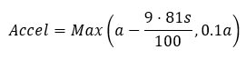
Where:

• a = the desired acceleration calculated by Gipps
• s = the slope as expressed as a percentage gradient.

Slope units are expressed as a percentage. To avoid zero or negative acceleration values, the minimum value is set to be 10% of the maximum desired acceleration. If the section is flat (slope = 0), the maximum acceleration is not changed from the default value.

TWOPAS Acceleration and Slope Model

The TWOPAS acceleration and slope model simulates the impact of engine output, weight, air resistance, and slopes on a vehicle’s speed and acceleration. Unlike the default slope model, this model also affects vehicle movements in flat locations because it gives a more detailed acceleration profile for a vehicle than the default Gipps model. The enhanced detail comes from the consideration of engine output, weight, and air resistance.

This model applies when the dynamic experiment's Behavior tab has Apply TWOPAS Slope Model ticked, and if the vehicle type's Dynamic Models tab has Speed on Slopes Affected by Weight (TWOPAS Model) ticked. It overrides the speed and acceleration values calculated using the Gipps model.

The TWOPAS acceleration and slope model was implemented using equations 9 and 10 from pages 34 and 35 of Capability and Enhancement of the VDANL and TWOPAS for Analyzing Vehicle Performance on Upgrades and Downgrades With IHSDM (Report FHWA-RD-00-078, 2000).

Note that these formulas were originally designed for vehicles weighing over 10 tonnes. However, it is possible, with care, to use the TWOPAS model for all vehicle types.

The acceleration on up gradients is calculated as follows.

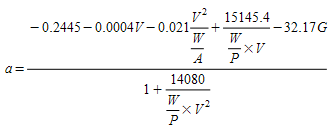
Where:

• V is the current speed in feet/s

• G is the angle of the slope in radians

• W/P is the weight-to-power ratio in lb/hp

• W/A is the weight-to-front-surface ratio in lb/ft².

The crawl speed is obtained by solving the equation for a = 0 numerically. At this point the maximum speed is limited to the crawl speed because the level of resistance from the air and the slope equals the engine output. However, it does not give a detailed crawl speed for downhill slopes for heavy vehicles. For this purpose, the downhill crawl-speed model should be used (see the next section).

Downhill Crawl-Speed Model for Heavy Vehicles

The downhill crawl-speed model for heavy vehicles simulates the impact of downhill slopes on a vehicle’s speed. It uses the vehicle’s weight, the severity of the slope, and the length of the slope. It is designed to be used for heavy vehicles which use a smaller gear when going downhill and reduce their speed to avoid their brakes overheating.

The maximum speed is calculated using equation 35 on page 83 of Feasibility of a Grade Severity Rating System (Report FHWA-RD-79-116, 1980) as follows.

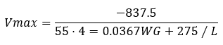
Where:

• Vmax is the maximum speed in mph

• W is the weight in lbs

• G is the angle of the slope in radians

• L is the length of the downhill slope in miles

Note that the total length of the down gradient is taken into account. Aimsun Next takes the length of each section to perform this calculation, so it is very important not to split the downhill slope across separate sections, if possible.

To ensure consistency between uphill and downhill slopes, the minimum downhill crawl speed is set to match the crawl speed for an uphill section of the same slope. If the desired speed is less than the downhill crawl speed, then the desired speed is used.

For this reason, the model would not change the downhill speed for most vehicles. It would only change the vehicle’s downhill speed where the weight of the vehicle is very heavy and on a very steep slope that is very long (e.g. 40 tonnes on a three-mile downhill section with a 7% slope).

For mesoscopic models, see Tuning Modeling Parameters in the Mesoscopic Simulator.

Influence of Global Parameters

The number of parameters that need to be set for a mesoscopic experiment is much smaller than those needed for a microscopic experiment. However, there is also an option to include the TWOPAS acceleration and slope model to simulate the impact of uphill and downhill sections.

It does so by limiting the uphill and downhill crawl speeds to the speeds calculated by TWOPAS and other downhill crawl-speed models. For more information, see TWOPAS Acceleration and Slope Model.

Microscopic Free-flow aCceleration Model (MFC)

The MFC model (sometimes referred to as the Microscopic Free-flow aCceleration Model) is a backward-looking model, deducing acceleration and deceleration from vehicle speed and from each component used in the operation of the vehicle. The MFC model is based on these two papers:

Makridis M, Fontaras G, Ciuffo B, & Mattas K. "MFC Free-Flow Model: Introducing Vehicle Dynamics in Microsimulation", Transportation Research Record, 2019; 2673(4): 762-77, doi:10.1177/0361198119838515.

He Y, Makridis M, Mattas K, Fontaras G, & Ciuffo B, Xu H. Introducing Electrified Vehicle Dynamics in Traffic Simulation, Transportation Research Record, 2020; 2674(9): 776-791, doi:10.1177/0361198120931842.

This model assumes free-flow conditions and applies the following principles at crucial stages:

• As a vehicle approaches the vehicle in front, its maximum acceleration is applied until the vehicle in front becomes the leader in the car-following model.
• At yield/give way controls, acceleration is taken into account when calculating the time required to reach and pass these points.
• At traffic lights, the MFC model is applied to the first vehicle only, unless there are large gaps between vehicles, when it will be applied to a second, distant, vehicle and so on. For vehicles accelerating on a green light it affects the rate at which vehicles pass the signal and how they reach their desired speed, where speed limits permit.

Reaction times play no part in any of our acceleration models because Reaction Time is a restricted parameter of the car-following model. They also have no effect on the lane-changing model because traffic conditions are based on desired speed.

The MFC model is able to capture, accurately and consistently, the acceleration dynamics of road vehicles using a lightweight approach. It averages vehicle parameters by vehicle categories and takes into account the different road conditions and driver behavior that are set in Aimsun Next. The MFC requires the following inputs:

• Vehicle

• Vehicle category (defined by vehicle type)

• Engine type (defined by the fleet composition of the vehicle type)

• Segment (taken from the Weight parameter distribution)

• Driver behavior

• Gear-shifting (defined by the headway aggressiveness of the vehicle type)

• Driving style (defined by the headway aggressiveness of the vehicle type)

• Road conditions

• Slope (defined by the segment of the section: P1, P2, P3, etc.)

• Weather (defined on the scenario's Parameters tab)

You can set the vehicle category in the Vehicle Type dialog. Here you can also set the engine-type composition. The vehicle segment is set for each vehicle with reference to its Weight distribution, which you can set in the Vehicle Type dialog > Dynamic Models > Main subtab. Currently, only the following segments for the Car category are included: A, B, C, D, E, F, J, N/M (for more information, see the Wikipedia article Euro Car Segment). The Euro Car Segment is set by the weight of the vehicle generated. The distribution of the Euro Car Segment by Engine Type and by Weight (in kilograms) is as follows:

• Petrol:

  A (800–999), B (1000–1179), C (1180–1299), D (1300–1589), E (1590–1749), F (1750–2600), J (1180–2600), N/M (1180–2600)

• Diesel:

  A (800–999), B (1000–1199), C (1200–1379) D (1380–1599), E (1600–1849), F (1850–2600), J (1200–2600), N/M (1200–2600)

• Electric:

  A (800–1249), B (1250–1459), C (1460–1699) D (1700–2099), E (2100–2449), F (2450–2600), J (1460kg–2600kg), N/M (1460kg–2600kg)

You will notice that some weights in C, D, E, and F overlap with equivalent weights in J and N/M. This means that if you set one of the first four categories, you might also pick up some vehicles from J and N/M. The segment set is based on the following sales distribution percentage: 35% are C, D, E, and F (depending on Weight), 25% are J, and 40% are N/M.

With these three inputs (category, engine type, segment), Aimsun Next can set the proper internal parameters of the engine of each vehicle and define default curves that relate speed and acceleration, taking into account the parameters of different vehicles.

Driver behavior is represented in the model by gear-shifting and driving style, which both help to define the headway aggressiveness of vehicles.

Gear-shifting strategy correlates the shifting points when the driver changes gear with the power curve of the vehicle and thus the operating speed of the vehicle’s power train. Driving style defines the amount of potential acceleration that a driver can use.

Moreover, the model includes the resistance forces acting upon the motion of the vehicle. You can define the slope in the Section dialog and set Weather conditions on the experiment's Parameters tab. The weather affects the friction coefficient of the road and thus the maximum tractive force of the vehicle in every time-step.

The model takes the full-load curve of combustion engines and the power curve of electric engines to calculate the potential acceleration versus the speed curve. From these fundamental curves, the model obtains the final acceleration and deceleration values, by considering the resistances which depend on environmental conditions. Also, the model applies a driving-style factor to the final acceleration and deceleration.

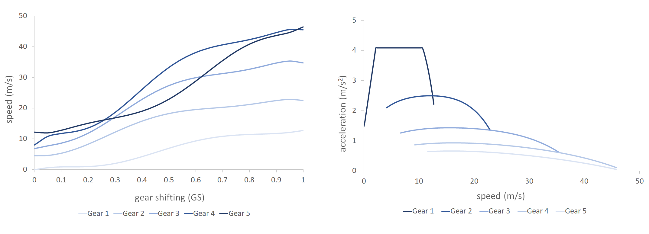
In the case of combustion engines (petrol and diesel), manual transmission is used, so it also includes limits on speed due to gear-shifting, which depends on driver behavior. The following curves are the MFC curves for a given road condition for a Petrol-Euro Car Segment A vehicle. The deceleration curve is the same as acceleration, but the driving-style factor applied is different:

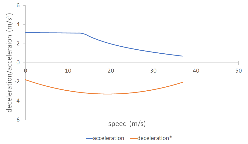
This next example concerns electric vehicles and shows the Electric-Euro Car Segment A curves. In this case, the deceleration curve is a synthetic curve obtained and extended for different vehicle profiles. It is taken from the validation test in the paper by He et al., 2020:

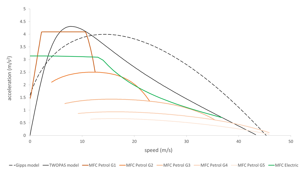
Finally, to compare complex and simpler models, here is an acceleration/speed curve of all the acceleration models included in Aimsun Next for a similar vehicle profile (Gipps is the car-following model):

Driver Parameters

Driver Reaction Time

This is the time it takes a driver to react to speed changes in the preceding vehicle. It is used in the car-following model. The Reaction time can be either Fixed (equal to Simulation Step) or Variable (multiple of Simulation Step). In case of Fixed, it is the same value for all vehicles. In case of Variable, the user can define a discrete probability function for each vehicle type (see Figure below). Note that for each vehicle type, the sum of probabilities must be 1.0. The Reaction Time for every individual vehicle will be sampled from this distribution.

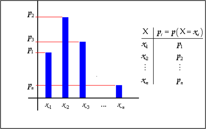
Example:

• Vehicle Type Car
• Values of Reaction Time: x1=0.6, x2=0.7, x3=0.8
• Probabilities: p1=0.2, p2=0.7, p3=0.1

The Reaction Time assigned to a vehicle is fixed for that vehicle but can be adjusted in particular sections by editing the “Reaction Time Variation” for the section through the Table View. The reaction time of a vehicle in a section is calculated as:

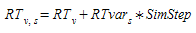
where:

• RT~v,s~ is the reaction time of vehicle v at section s
• RT~v~ is the reaction time of vehicle v
• RTvar~s~ is the reaction time variation in section s
• SimStep is the simulation step

Reaction time at Stop and Reaction time at Traffic Light

The vehicle reaction times are set in the Experiment Editor: Reaction Times Tab and can be set for all vehicle types of set individually for different vehicle types.

• Reaction time at stop is the time it takes for a stopped vehicle to react to the acceleration of the vehicle in front.

• Reaction time at traffic light is the time it takes for the first vehicle stopped after a traffic light to react to the traffic light changing to green.

Reaction time at stop is used as reaction time only for vehicles that start from a stopped condition, while the normal reaction time is used for vehicles that are moving. The reaction time at stop has a strong influence in the queue discharge behavior and it therefore gives the user a strong calibration parameter in queue modeling.

Queue Speeds

The speeds which control whether a vehicle is marked as being in a queue are set in the Experiment Editor: Behavior Tab.

Queue Entry Speed

Vehicles whose speed decreases below this threshold value (in m/s) are considered to be stopped and consequently in a queue. This parameter affects statistical data gathering for stops and queues. Whenever the speed of a vehicle decreases below the queue entry speed a new stop for that vehicle is added to the number of stops statistic. Same stop will be considered while the speed remains below the queue exit speed parameter. Once the vehicle speed goes above the queue exit speed parameter it is no longer considered in a queue nor stopped. A new stop will be added to the number of stops statistics when the vehicle speed goes below queue entry speed again.

Queue Exit Speed

Vehicles that are stopped in a queue whose speed increases above this threshold value (in m/s) are considered to have left the queue and no longer to be at a standstill. This parameter affects statistical data gathering for stops and queues.

Queue Entry and Queue Exit Speed parameters also have an influence on the lane-changing model. A vehicle driving in zone 3 of a section is not willing to wait for a gap for longer than the Maximum Yield Time plus the Additional Waiting Time Before Missing Turn at a standstill and the condition of standstill is determined by these parameters.

Global Simulation Parameters

Simulation Step

The system update time interval, also called the cycle. At every simulation step, the state of all the elements of the system are updated (i.e. vehicles and events such as traffic light changes). The Simulation Step can range from 0.1 to 1.5 seconds and can be different from the Reaction Time parameter.

Rule of the Road

When editing a network, the user can define whether the vehicles drive on the left or on the right side of the road, as a global parameter for the whole network. This parameter is taken into account in the lane-changing model as follows:

• When a vehicle attempts to overtake another vehicle it will try to do so using the adjacent left lane when driving on the right side, or the adjacent right lane when driving on the left.
• When a vehicle is driving fast enough and wants to move back to the slower lane, it will try to go to the rightmost lane when driving on the right and to the leftmost lane when driving on the left.
• When a vehicle enters the network via a section, it will prefer to use the rightmost lane when driving on the right and the leftmost lane when driving on the left.

As a result of this modeling, in a left-hand driving network, vehicles tend to drive using the leftmost lane of the sections and in networks driving on the right, vehicles tend to prefer the rightmost lanes. The effect of this parameter on simulation results varies, depending on the geometry and type of the network (urban or interurban), but it always affects the behavior of the vehicles.

Distinguish destination lanes in turns

This parameter states whether or not the user is able to specify the possible destination lanes when defining a turn movement.

When this parameter is set to NO, it is assumed that all lanes of the destination section in a turn are possible. This means that, when defining a turn, the user can choose the origin section, the lanes from this section where the turn is allowed and the destination section, but not the lanes of the destination section. If this parameter is set to YES, when defining a turn the user can choose, not only the lanes from the origin section where the turn will be allowed, but also the lanes in the destination section. When a vehicle makes a turn it will then be able to use only the specified lanes, both for the origin and destination sections.

These two parameters are edited in the Preferences Editor.