Arrivals

Arrivals Algorithms

The time interval between two consecutive vehicle arrivals (the headway) is sampled from a random distribution – a headway model. When loading a traffic demand into the simulation, that is either a set of traffic states or a set of OD matrices, the different headway models are: exponential, uniform, normal, constant, “ASAP”, and external. ‘Exponential’ is the default distribution. The generation model is set globally on a per scenario basis; however, it can be overridden for individual centroids in the case of OD traffic demand, or for individual sections in the case where demand is a traffic state. Vehicles generated from a traffic arrival use the generation time defined in the traffic arrival to enter the network.

The Traffic Generation distribution can be selected from: Exponential, Uniform, Normal, Constant, External, and ASAP.

Exponential

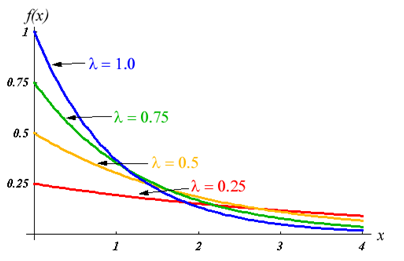
Time intervals between two consecutive vehicle arrivals (headway) at input sections are sampled from an exponential distribution (Cowan 1975). The mean input flow (in vehicles/second) is λ, and the mean time headway is calculated as 1/λ seconds.

The algorithm for calculating the time headway (t) is the following:

u = random (0,1)
if (lambda > 0.0)
    t = ((-1/lambda)*ln(u))
else
    t = max_float
endif

Uniform

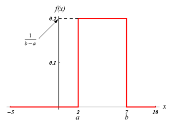
Time intervals between two consecutive vehicle arrivals (headway) at input sections are sampled from a uniform distribution. The mean headway (T) is taken as 1/λ seconds, λ being the mean input flow (in vehicles/second) and the range used for the distribution is [T-T/2, T+T/2].

The algorithm for calculating the time headway (t) is the following:

if (lambda > 0.0)
    T = 1/lambda
    u = random (0,1)
    minU = -T/2
    maxU = T/2
    t = T+[minU+(maxU-minU)*u]
else
    t = max_float
endif

Normal

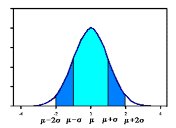
Time intervals between two consecutive vehicle arrivals (headway) at input sections are sampled from a truncated normal distribution. The mean headway (T) is taken as 1/λ seconds, where λ is the mean input flow (in vehicles/second) and the variance (σ) is taken as 10% of the mean. The range of the truncated normal is [T-2σ, T+2σ].

The algorithm for calculating the time headway (t) is the following:

if (lambda > 0.0)
    T = 1/lambda
    n = t_normal (1,0.1)        (truncated normal)
    t = maximum [error, n*T]    (error ->0, error > 0)
else
    t = max_float
endif

Constant

Time intervals between two consecutive vehicle arrivals (headway) at input sections are always constant. The headway (t) is taken as 1/λ seconds, λ being the mean input flow (in vehicles/second).

The algorithm for calculating the time headway (t) is the following:

if (lambda > 0.0)
    t = 1/lambda
else
    t = max_float
endif

ASAP

In this generation model, vehicles are entered in the network ‘as soon as possible’, i.e. as soon as there is some space available in the input section. This model is intended to make the most use of the network entrance capacity. It could be used, for example, for simulating evacuation situations. In this case, no headway is generated. At the beginning of each time slice, the total flow to be input during the slice is ‘piled up’ at the entrance section and vehicles are entered into the section one after the other as soon as the previous one has left enough space in the case of microsimulation and has the minimum headway in the case of mesoscopic simulation.

External

This option allows the user to introduce the vehicles into the network via the Aimsun Next API. No vehicles are generated or input into the network via any section by the simulator itself. Therefore, an external DLL, user-defined program, is required to insert vehicles into the network.

Summary of Generation

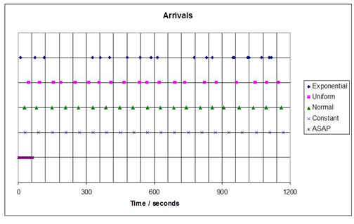
The next figure shows a comparison of traffic generation models for a 20 minute period. The results are for a demand of 60 vehicles over one hour onto a link in free flow.

Dealing with Fractional Numbers of Trips

When the OD demand in a time slice has a fractional number of trips, the demand in that slice is rounded to an integer demand with the probability of being rounded up or down proportional to the fractional value. Hence, for example, a stated demand of 22.8 in an OD matrix cell will give a requested demand of 22 with a 20% probability or 23 with an 80% probability, similarly a stated demand of 0.6 will give a requested demand of 0 with a 40% probability or 1 with a 60% probability.

Taken over a large number of OD pairs, the total demand in the model replication will closely match the overall total demand, although an exact match is not guaranteed.

For each OD cell in each time slice, the release algorithm for all Arrivals modes, apart from ASAP is:

EventTime = SliceStartTime;
AvgHeadway = SliceDuration / RequestedDemand
ShiftedTime =  RandomBetween (0, (SliceEndTime-SliceStartTime)) + AvgHeadway;
MaxTime = SliceEndTime + ShiftedTime;

while (Continue) {
    MyHeadway = getRandomisedHeadway(ArrivalsModelType, AvgHeadway);
    EventTime = EventTime + MyHeadway;
    if ( EventTime >= (SliceStartTime+ShiftedTime) and EventTime < MaxTime) 
        AddVehicleArrival( EventTime-ShiftedTime, ... );
        TotalReleased++;
        Continue = (EventTime < MaxTime);
    endif
endwhile
return TotalReleased

Where

• AvgHeadway: is the mean headway between arrivals.
• RequestedDemand: is already an integer.
• MyHeadway: is a randomized headway according to the arrivals model in use.
• ShiftedTime: is used to set an offset to randomize the release times.
• EventTime: is the time set for the release.
• SliceDuration, SliceStartTime, and SliceEndTime: are the length, start, and finish times of the OD time slice, but note that the end time will be capped to the simulation duration and the difference between these two values might not be the same as SliceDuration in the last slice.

The ShiftedTime variable offsets the timing of the arrivals sequence by a random time in the range AVGHeadway to AvgHeadway + Actual Length of Slice. The goal is to shift the start of the sequence to a random point in time. Without this shift, in the Constant release mode where vehicles arrival at regular intervals, the arrivals would cluster around the fractional divisions of the slice time creating artificial peaks in the number of vehicles arriving in the network. Shifting the apparent base time of the slice for the sequence of releases and only taking those which occur in this shifted time prevents this occurring. The same shift process is then applied for all arrival modes, with the exception of ASAP.