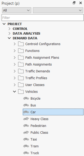
Vehicle Types

A vehicle type is a classification of vehicles and drivers with common physical and behavioral characteristics. For instance, types such as car, taxi, public bus, private bus, LRT (Light Rail Transit), SUV (Sport Utility Vehicle), truck, and long truck can be defined.

Use the Project menu or the Demand Data context menu to create a new Vehicle Type. They can also be created from their own folder context menu.

Vehicle Classification

Vehicles types can be grouped into Vehicle Classes.

Vehicle Classes are only used in reserved lane definitions. For example, Public, Private, Emergency, and HOV (high occupancy vehicle) classes, which correspond to reserved lanes definitions in the network model. The use of Classes is optional and is only required when there are lane restrictions.

Vehicle Types refers to the different kinds of vehicles for which the traffic demand data is defined. This includes input flows and turn proportions as well as the number of trips in the OD matrices which can be specified for each vehicle type. The use of vehicle types in a model is required to define traffic demand data. Vehicle types are also use to define the physical characteristics of the vehicle such as width, length, speed, acceleration, deceleration, and its appearance.

A Class can be composed of one or more Types and a Type can belong to none, one, or several Classes. For example:

• Public Class: bus, taxi, ambulance, police car
• Private Class: car, HGV, truck, van, HOV car
• Emergency Class: ambulance, police car
• HOV Class: HOV car
• Car class:car, police car, HOV car
• Commercial Class: HGV, truck, van

A reserved lane can be defined for a certain class. For instance, a reserved lane can be defined for the public class. This lane would only be available for buses, taxis, ambulances, and police cars using the example above.

Vehicle Type Editor

The vehicle type editor is used to specify the physical characteristics and the parameters of a type of vehicle. Setting appropriate values for these parameters is part of the model calibration process.

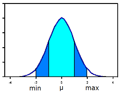
Almost all parameters are defined using a truncated normal distribution.

Main Tab

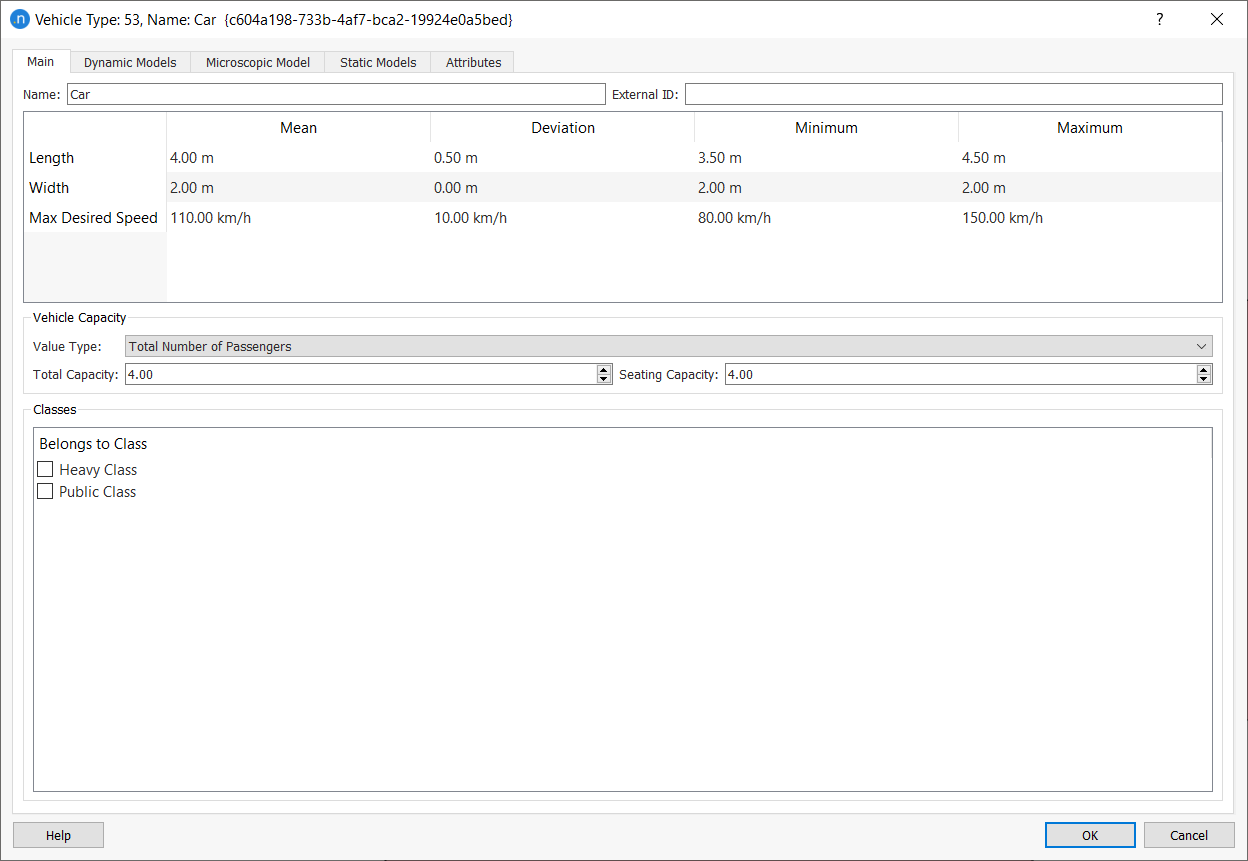
In the Main tab, the vehicle type’s Name and External ID is defined. Also the vehicle type’s physical parameters such as Length, Width, and Maximum Desired Speed are defined.

Length

The length, in meters, for this type of vehicle. This parameter is used both for graphical and modeling purposes. It has a direct influence on traffic modeling, as vehicle length is taken into account in microscopic and mesoscopic vehicle behavior models.

Width

This is the width, in meters, for this type of vehicle. This parameter is only used for graphical purposes and does not have a direct influence on the traffic modeling.

Maximum desired speed

This is the maximum speed, in km/h, for this type of vehicle when not otherwise constrained by section speed limits. For example, a ‘car’ vehicle type with a maximum desired speed of 110 km/h, a deviation of 10 km/h, a maximum value of 140 km/h and a minimum value of 90 km/h could be defined. Car speeds would be sampled from a Normal (110,10) distribution in a microscopic or mesoscopic simulation. A 'sports car' type could also be defined with much higher speed potential

Maximum Capacity

This denotes the maximum number of passengers that can travel in a vehicle of this vehicle type. This value can be set either as a multiplying factor of vehicle length or as a total value. This parameter is used by the pedestrian simulator when loading pedestrians into transit vehicles and also in the Transit Assignment. Refer to the Pedestrian Simulator manual or Travel Demand Modeling for more information.

Vehicle Classes

The vehicle type can be associated with any of the existing vehicle classes by selecting the desired class in the Classes folder. See the Vehicle Class Editing section for details on creating vehicle classes.

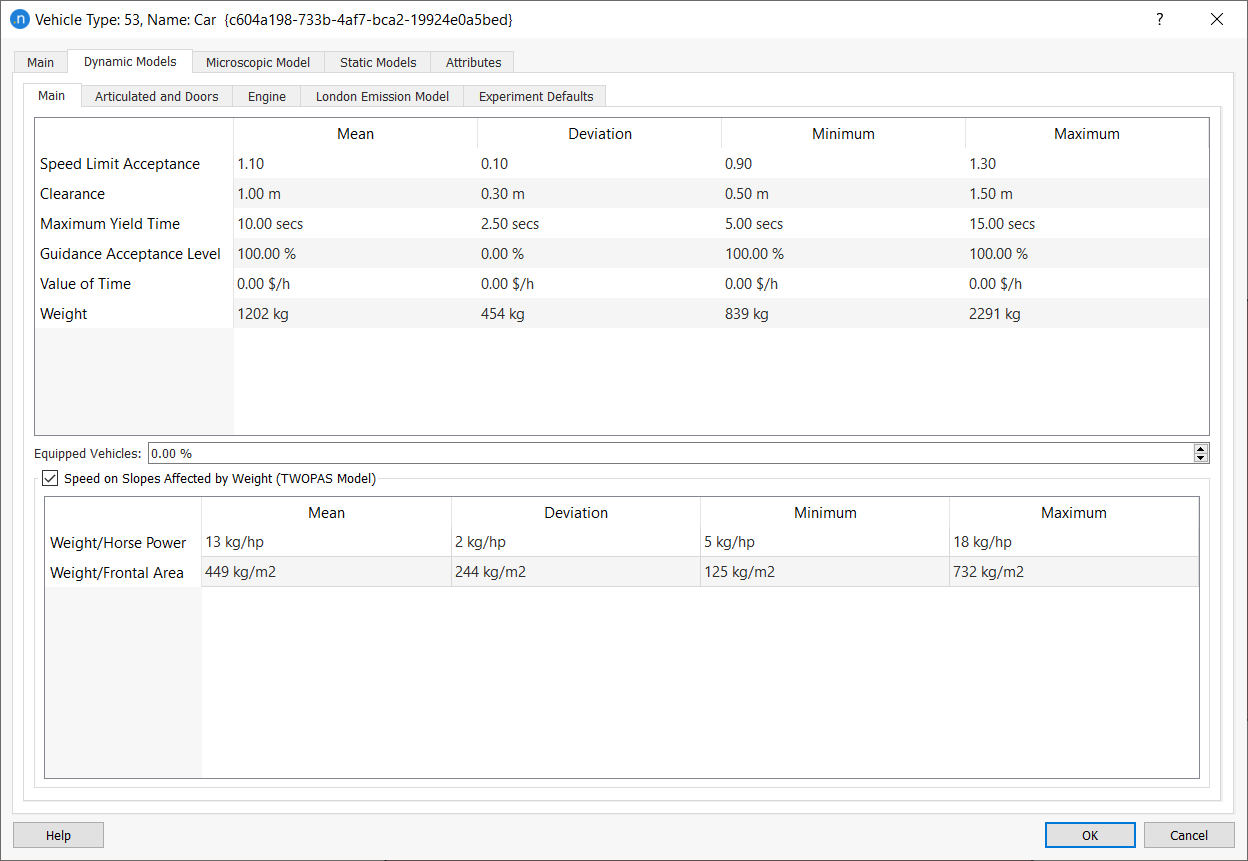
Dynamic Models Tab

This tab holds the parameters that are used by the microscopic and mesoscopic simulators. Almost all parameters are defined using a truncated normal distribution.

Speed Limit Acceptance

This parameter can be interpreted as the ‘level of goodness’ of the drivers or the degree of acceptance of speed limits. When is greater than 1 means that the vehicle will take as maximum speed for a section a value greater than the speed limit, while when is lower than 1 means that the vehicle will use a lower speed limit. See the next section for details on how the maximum desired speed for a vehicle is calculated for different parts of the network.

Clearance

This is the distance, in meters, that a vehicle keeps between itself and the preceding vehicle when stopped.

Maximum Yield Time

When a vehicle is in a yield situation, for example at a Yield or Stop sign in a junction or an on-ramp in a freeway, it applies either the normal gap-acceptance model or a lane-changing model in order to cross or merge with traffic, respectively. When a vehicle has been at a standstill for more than this Yield Time (in seconds), it will become more aggressive and will reduce the acceptance margins. This period is also used in the Lane-Changing model as the time that a vehicle accepts being at a standstill while waiting for a gap to be created in the desired turn lane before giving up and continuing ahead.

Guidance Acceptance Level

This parameter, between 0 and 1, gives the level of compliance of this vehicle type with the guidance indications, such as information given through Variable Messages Signs or particular Vehicle Guidance Systems. This parameter represents the probability that a vehicle will follow a recommendation. In current version of Aimsun Next, it is considered only for traffic management actions (In previous versions this parameter was used to determine the number of guided vehicles for the Dynamic Traffic Assignment. In the current version the number of guided vehicles is determined by the en-route path update percentages defined in the experiment).

Value of Time

This parameter is only used in user defined route choice functions to define a value of time. It gives the conversion from monetary cost to time, so units can be $/h, €/sec, etc.

For example, to add the cost of tolls to a cost function where the cost is based on section length, a tollPrice, and the vehicle value of time, the following code would be used:

def cost(context, manager, section, turning, travelTime):
    sectionSpeed = min(
        section.getSpeed()*manager.getNetwork().getVehicleById(context.userClass.getVehicle().getId()).getSpeedAcceptanceMean(),
        manager.getNetwork().getVehicleById(context.userClass.getVehicle().getId()).getMaxSpeedMean())
    turnSpeed = min(
        turning.getSpeed()*manager.getNetwork().getVehicleById(context.userClass.getVehicle().getId()).getSpeedAcceptanceMean(),
        manager.getNetwork().getVehicleById(context.userClass.getVehicle().getId()).getMaxSpeedMean())
    attractivityFactor = 1+manager.getAttractivenessWeight()*(1-turning.getAttractiveness()/manager.getMaxTurnAttractiveness())
    res = (section.length3D()/sectionSpeed+ turning.length3D()/turnSpeed)*attractivityFactor
    res = res + manager.getUserDefinedCostWeight()*section.getUserDefinedCost()
    tollPrice = 10  #units in monetary cost per meter taking also into account time units of VoT
    vehicle = context.userClass.getVehicle()
    res = res + (section.length3D()+turning.length3D())*tollPrice/vehicle.getValueOfTimeMean()
    return res

Weight

This parameter defines the vehicle weight, that is used in the LEM emissions model.

Equipped vehicles

This is the percentage of vehicles that are 'Equipped'. Equipped vehicles can be detected by detectors with measuring capability ‘Equipped’, which provide the detection time, the detector identifier, the vehicle identifier, the vehicle type name, and the transit line identifier if it is a transit vehicle.

Speed on Slopes Affected by Weight (TWOPAS Model)

The parameters Weight/Horse Power and Weight/Frontal Area are required when the TWOPAS slope model is activated in the dynamic simulation.

However, if the other Aimsun Next microsimulator acceleration model – the MFC – has been activated, this group box is disabled. This is because our acceleration models are exclusive. You can activate or deactivate the MFC acceleration model in the Vehicle Type dialog > Microscopic Model > Car Following subtab by ticking or unticking Apply MFC model.

In mesoscopic simulations, the formula that gives the uphill crawl speed is used to limit the maximum speed of the vehicle. The formula for downgrades gives a maximum speed, so it can be directly applied in mesoscopic simulations.

Articulated and Doors

You can find the Articulated and Doors subtab on the Dynamic Models tab of the Vehicle Type dialog.

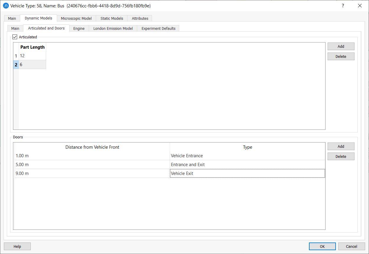
Articulated Vehicles

To set as an articulated vehicle:

1. Tick the Articulated box.
2. Click Add to add articulated sections to the vehicle and input values for each Part Length.
3. If you need to remove articulated sections, select a section and click Delete.

Doors

To set the vehicle's doors:

1. Click Add and select a Type from the drop-down list.
2. Input a value for Distance from Vehicle Front for the door.
3. Repeat step 2 for additional doors if required.
4. Click OK to save your changes.

This information will only be used by transit vehicles when simulating pedestrians. For more information about how doors are simulated in micro and mesosimulations, see Vehicle Attributes and Behavior of Transit Stops.

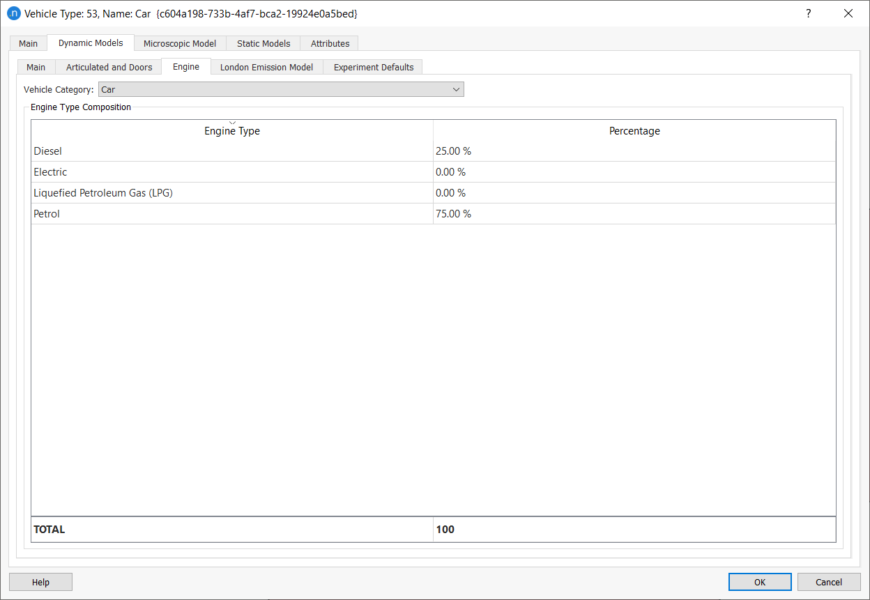
Engine

The Engine tab contains the Vehicle Category and Engine Type Configuration parameters. These are used by the microscopic and mesoscopic simulators.

Vehicle Category describes the particular vehicle type: car, commercial vehicle, bus, motorbike, or non-motorized. Engine Type Composition enables you to define the percentages of engine types (Diesel, Electric, Liquefied Petroleum Gas, and Petrol) in the fleet configuration for the vehicle type.

Both these parameters enable you to define different vehicle profiles in the MFC acceleration model, Energy (Fuel and Battery) Consumption Models, and emission models (QUARTET, Panis et al., and LEM).

The Experiment Defaults tab allows parameters to be edited that can be later on changed at experiment level. These parameters here are in effect a template, allowing the user to change in the experiment only those required for calibration. It includes the driver’s reaction times and parameters related to the dynamic traffic assignment.

There are three different reactions times in microscopic simulation:

• Reaction time: This is the time it takes a driver to react to speed changes in the preceding vehicle.

• Reaction time at stop: This is the time it takes for a stopped vehicle to react to the acceleration of the vehicle in front.

• Reaction time at traffic light: This is the time it takes for the first vehicle stopped after a traffic light to react to the traffic light changing to green.

In mesoscopic simulation only the reaction time and reaction time at traffic lights are used.

Different reaction times can be defined associating a probability between 0 - 1.0 to each of them . All the reaction times probabilities must total 1.00

The role of the reaction time, the reaction time at stop, and reaction time at traffic light parameters is documented in the Parameters section in the Vehicle-based Simulators theory section of the manual.

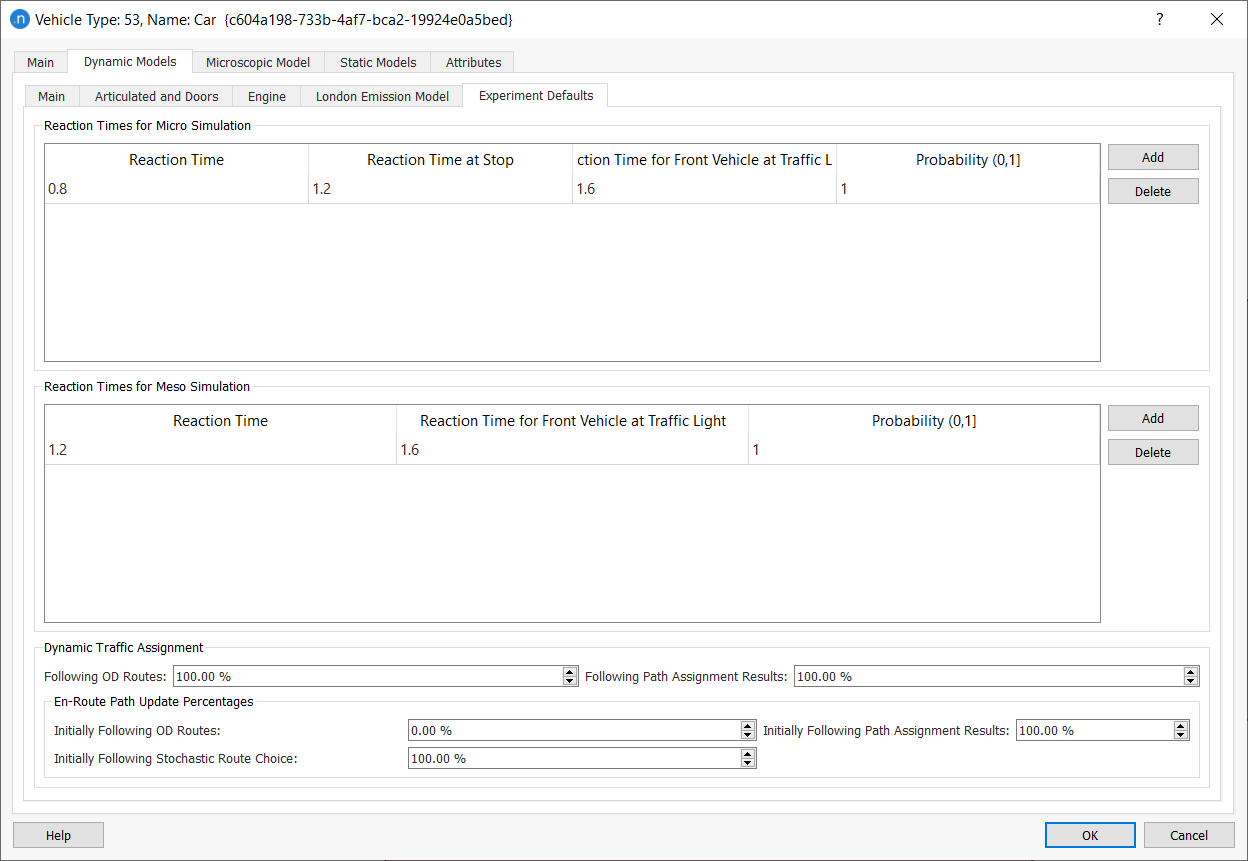
The default dynamic traffic assignment parameters that can be defined are:

• Following OD Routes: Defines the percentage of vehicles belonging to this vehicle type that will try to follow an OD Route (user-defined route) when entering the network.

• Following Path Assignment Results: Defines the percentage of vehicles belonging to this vehicle type that will try to follow a route from the Path Assignment results file, when entering the network.

• Path Update for Vehicles Using OD Routes: Defines the percentage of this vehicle type that follow an OD Route (user-defined route) and might have their path re-assigned. See the section on Stochastic Route Choice, En-Route Path Assignment Update.

• Path Update for Vehicles Using Path Assignment Results: Defines the percentage of vehicles belonging to this vehicle type that follow a route from the Path Assignment results file given as input might have their path re-assigned.

• Path Update for Vehicles Using Route Choice Models: Defines the percentage of vehicles belonging to this vehicle type that follow a route from the Route Choice Models and might have their path re-assigned.

There are three different kinds of paths a vehicle can be assigned when entering the network: OD Routes (user-defined routes), Path Assignment Result and Calculated Shortest Paths using the Route Choice Model. The “Following OD Routes” and “Following Path Assignment Results” percentages determine the probability of use of each of the three options and they do not have to add up to 100%. OD Route percentage is the first value to be considered when a vehicle enters the network. If the probability states that the vehicle will be assigned with an OD Route, then Aimsun Next will look for a path according to percentages and routes defined by the user. If the vehicle is not assigned to an OD Route, then the probability of being assigned with a path from Path Assignment object imported into the scenario (if any) is applied. Finally, if the vehicle is not assigned with an OD Route, nor with a Path Assignment result, a choice from the DTA Paths calculated by Aimsun Next is applied.

For example, if the assignment was 60% ‘Following OD Routes’ and 70% ‘Following Path Assignment Results’, 60% of the generated vehicles will follow an OD route, 28% (70% * (100% - 60%)) will follow a path read from a path assignment file and 12% (100% - 60% - 28%) will follow a path built by the route choice model. This is on the basis that for each OD pair there is a route defined in the OD Matrix Path Assignment tab and a route in the path assignment file.

Refer to the Stochastic Route Choice section for more details about the use of these percentages.

Microscopic Model Tab

Main Parameters

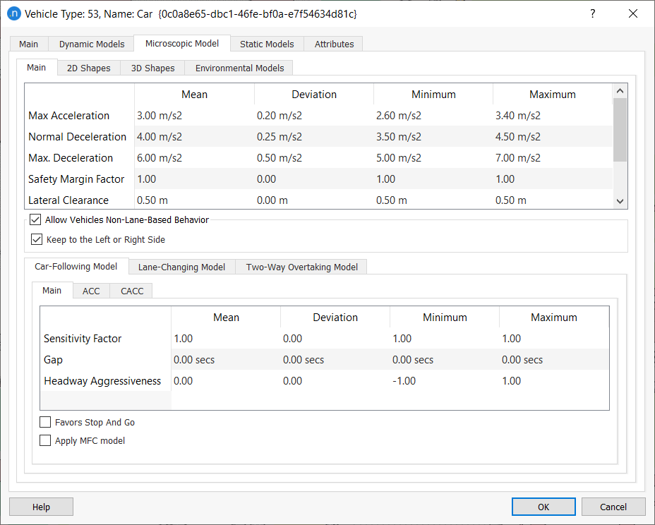
The parameters in this subtab control the behavior of the vehicles in the simulation; refer to the Behavioral models section for more details.

Maximum Acceleration

This is the maximum acceleration, in m/s2, that the vehicle can achieve under any circumstances. This acceleration is as used in the Gipps car-following model (see Gipps, 1981 and 1986b).

Normal Deceleration

This is the maximum deceleration, in m/s2, that the vehicle can use under normal conditions. This deceleration is as used in the Gipps car-following model.

Maximum Deceleration

This is the most severe braking, in m/s², that a vehicle can apply under special circumstances, such as emergency braking for e.g. in front of a traffic light.

Safety Margin Factor

In the gap acceptance calculations to determine when a vehicle can move at a priority junction, the safety margin is set in the Road Type turn parameters. It can be modified for a specific turn to reflect the road geometry and can further be adjusted by vehicle type. This vehicle type parameter provides a multiplier, with a truncated normal range, to apply to the turn safety margin values.

Lateral Clearance

The lateral clearance vehicle to vehicle variations come from distributions defined by vehicle type. The minimum lateral spacing between two vehicles is the sum of the lateral clearances of both vehicles.

Max Lateral Speed

When moving laterally, the vehicles use their maximum lateral speed.

Allow Vehicles Non-Lane-Based Behavior

The Allow Vehicles Non-Lane-Based Behavior parameter controls whether the vehicle type can consider non-lane-based movements or not. For more information, see Non-Lane-Based Microscopic Simulation.

Note that if non-lane-based behavior is activated at the section level, it enables the consideration of lateral clearance in all traffic, that is for both non-lane-based vehicles and lane-based vehicles.

Keep to the Left or Right Side

In microsimulations, where Allow Non-Lane-Based Behavior for vehicles is activated, you can now instruct vehicles to stay close to the left or right side of the road, depending on the direction of travel. There is a new tick-box option in the Vehicle Type dialog named Keep to the Left or Right Side.

This new option is useful for modeling any vehicle that you want to stay close to the left or right side of the road, depending on the direction of travel. The instruction does not apply when vehicles need to cross lanes to turn right or left. Its obvious use is for bicycles but auto-rickshaws or any other type of vehicle can be instructed to behave in this way.

Car-Following Model

Car-Following Model: Main Tab

In the Main tab-folder of the Car-Following Model area, the default Aimsun Next car-following model parameters can be defined. They are:

Sensitivity Factor

In the deceleration component of the car-following model, the follower makes an estimation of the deceleration of the leader using the sensitivity factor.

Gap

This parameter is used to override the headway between vehicles as calculated by the car following model. The headway between two vehicles is defined as the distance in seconds between the front bumper of a vehicle and the front bumper of the following vehicle. The default Gap parameter value of 0.0 uses the distance calculated by the car-following algorithm. If a different value is used then the minimum of the Gap and the default distance is used. The application of this parameter is documented in the Microsimulation Theory: Car Following Algorithm section.

Headway Aggressiveness

The headway aggressiveness parameter modifies the relationship of the inter-vehicle distance as a function of speed. This distance is simply linear in the Gipps model and does not correspond to observed behavior under congested highway conditions. The modified car following model is documented in the Microsimulation Theory Section.

Favors Stop and Go

This option allows a vehicle to adjust how it uses the aggressiveness value. If the option is ticked the value +a is used during deceleration and of –a during acceleration. Hence, assuming a is positive, the gap between vehicles will be larger during acceleration than deceleration for the same speed.

Apply MFC model

This option activates the Microscopic Free-Flow Acceleration model (MFC). It might be disabled because the other acceleration model, the TWOPAS model, has already been activated. If you want to deactivate Speed on Slopes Affected by Weight (TWOPAS Model) you can do so on the Main subtab of the Dynamic Models Tab.

Car-Following model: ACC and CACC tabs

There are two additional car-following models for modeling autonomous and/or connected vehicles.

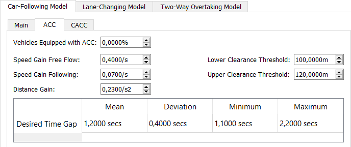
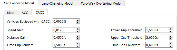
The distribution of non-equipped vehicles, ACC equipped vehicles, and CACC equipped vehicles is specified through the Vehicles Equipped with ACC percentage and Vehicles Equipped with CACC percentage each one located in the ACC and CACC tabs respectively. Those percentages should always sum up 100% at max, the rest being the non-equipped vehicles. As an example, having a 20% of Vehicles Equipped with ACC and a 30% of Vehicles Equipped with CACC will lead to a 50% of non-controlled vehicles in the network (human-driven vehicles).

Both types of vehicle, ACC and CACC, can perform Speed Regulation Mode, which is typically used when no vehicle is ahead of the current vehicle (or if vehicle ahead is too far).

ACC equipped vehicles use ACC Gap Regulation mode to control its movement based on the vehicle ahead if any.

CACC equipped vehicles use CACC Gap Regulation mode instead.

Note that when a vehicle is equipped with an ACC or CACC module, it will only be functional on roads whose road type allows it. Refer to the road type editor to activate the modules and specify the CACC vehicles platoon settings.

Refer to the Adaptive Cruise Control (ACC) and Cooperative Adaptive Cruise Control (CACC) car-following section for the explanation of the other parameters in these tabs.

Simulation vehicles have a new column on static attributes that is called ‘Cruise Control Capability’ to show which module, if any, is the vehicle equipped with. Values can be:

a. No Capability b. Adaptive Cruise Control (ACC) c. Cooperative Adaptive Cruise Control (CACC)

Simulation vehicles have a new a dynamic column that is called ‘Cruise Control Status’ to show which driving mode has been used in the last simulation step. The five possible values, detailed in the Decision Chart, are:

a. CC Speed Regulation b. ACC Gap Regulation c. CACC Platoon Leader Gap Regulation d. CACC Platoon Follower Gap Regulation e. Disabled

Lane-Changing model

Overtaking in Lanes

Parameters that affect lane changing and overtaking in parallel lanes are set by the Road Type and can be modified for individual Road Sections. These values can then be further modified by vehicle type to adjust behavior by type and, if a range is given, to randomize behavior for each vehicle.

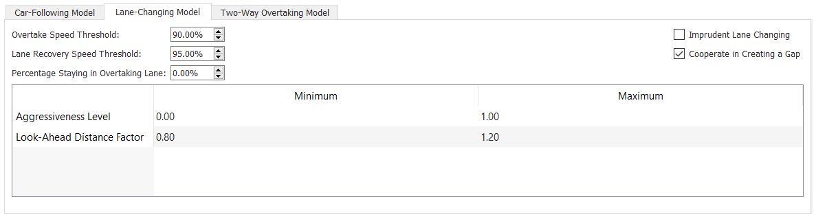
Overtake Speed Threshold and Lane Recovery Speed Threshold

These two parameters control overtaking maneuvers in Zone 1 when a vehicle changes lane to pass another. They are documented in the Microsimulation Theory Section.

If the vehicle is constrained to travel at less than Overtake Speed Threshold of its desired speed, it will consider an overtaking maneuver. Lane Recovery Speed Threshold is the percentage of the desired speed of a vehicle above which a vehicle might decide to get back into the original lane.

Percentage Staying in Overtaking Lane

Defines the probability that a vehicle of this type will stay in the faster lane instead of recovering to the slower lane after an overtake maneuver.

Imprudent Lane Changing

Defines whether a vehicle of this type will still change lane after assessing an unsafe gap.

Lane Change Gap Acceptance

If the Cooperate in Creating a Gap option is selected, vehicles of this type can cooperate in creating a gap for a lane changing vehicle to accept. With the option toggled on, the number of vehicles that effectively cooperate depends on the section cooperation percentage parameter.

Aggressiveness Level controls the Gap Acceptance Model for Lane Changing affecting the reduced gap a vehicle will accept to make a lane change. The higher the level, the smaller the gap the vehicle will accept, being a level of 1 the vehicle's own length.

Lane Change Look-Ahead

The Look-Ahead Factor is used to modify the look-aheads used in the Lane Changing Model to determine where vehicles consider their lane choice for a forthcoming turn. The default distances are set in the Road Type and can be modified for each turn to reflect local conditions in the Turn Editor. The zone distances can then be modified by a factor by vehicle type to adjust where lane changes start to be considered and, if a range is given, to randomize behavior for each vehicle of that type.

Two-Way Overtaking model

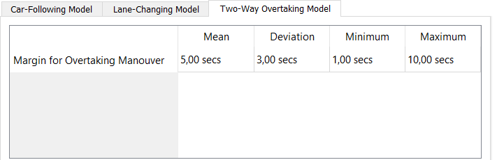
Margin for Overtaking Maneuver

The safety margin for two way overtaking is set here as a truncated normal distribution. The algorithms controlling the two way overtaking maneuver are described in the Microsimulation Theory: Two-way Overtaking Model Section.

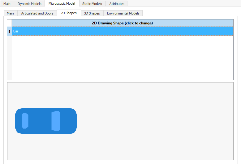
2D Shapes

In 2D views the microsimulation vehicles can be drawn in several ways (as car, bus, truck, long truck, van, bike, motorbike, pedestrian, box, circle, plane, rickshaw, auto rickshaw, cycle rickshaw, electric rickshaw, tractor, and trailer). Use the 2D Shapes folder to select the way all the simulation vehicles belonging to the current edited vehicle type will be drawn. If the current vehicle type has been defined as articulated, then a 2D Shape for each one of the articulated parts can be defined.

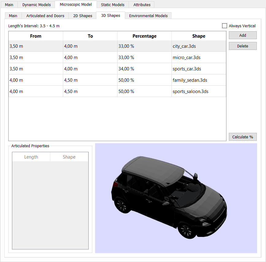
3D Shapes

In 3D views, the simulation vehicles are drawn using 3DS shapes. Click the 3D Shapes tab and select the 3DS shapes to use for simulation vehicles belonging to this vehicle type.

The Always Vertical option ensures that objects (vehicles and pedestrians, when relevant) keep their vertical aspect when moving on slopes. This should be unticked for road vehicles to ensure they follow the gradient as expected. It should be ticked for pedestrians, so that they move realistically, at the correct angle, for example when moving up and down stairs.

Environmental Models

All environmental model parameters are configured around the engine types of vehicles. You can set the percentages of engine types for vehicles in the Vehicle Type dialog > Dynamic Models > Engine subtab. Currently non-motorized vehicles and motorbikes are excluded.

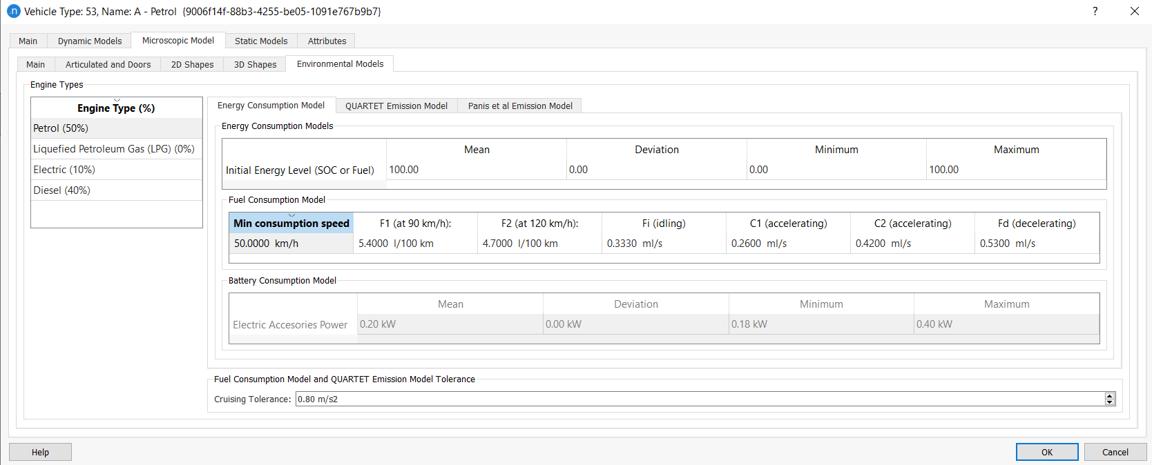
Energy Consumption

The energy consumption models include the Fuel Consumption Model for combustion engines and the Battery Consumption Model for electric vehicles. You can edit the parameters of both types of model for each type of engine of any vehicle type.

You can do this in the Vehicle Type dialog > Microscopic Model > Energy Consumption Models subtab. The ways in which these parameters are used are described in Fuel Consumption Model and Battery Consumption Model.

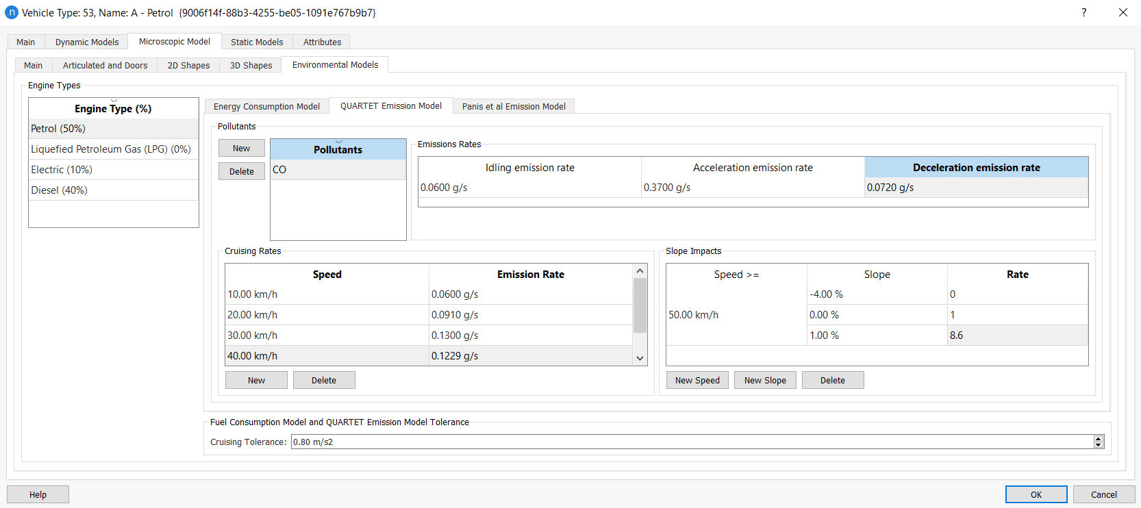
Quartet Emissions Model

On the QUARTET Emission Model subtab, the parameters of the QUARTET emission model are set by Engine Type (%). This utility is designed to produce a 'balance sheet' of all pollutants generated during the simulation.

When you create a pollutant for one vehicle type, it is automatically created for all other vehicle types and available for every engine type. Likewise, if you rename a pollutant, the change is applied across all vehicle types. This ensures that all vehicle types always have the same list of pollutants. Only the emission rates will differ between types.

To create a new pollutant, click the New button and enter the name and its three parameters. IER stands for Idling Emission Rate, AER and DER stand for Acceleration and Deceleration Emission Rates respectively. Speed dependent rates for this pollutant must be entered for at least one speed. Click the New button in the lower part of the dialog and enter the data.

Speed-emission rates are used for vehicles traveling at a constant speed. If the speed is not constant, then the IER, AER, and DER are used. If there is only one speed-emission pair for a pollutant, that emission rate will be used for all vehicles traveling at any constant speed. If there is more than one pair, the emission rates for vehicles traveling at a constant speed will depend on the speed intervals defined by the different pairs. The speed intervals are given by their upper limit. For example, if the speeds on the list are 10, 20, 30, 40, 50, 60, and 70 that the emission rate at constant speed has different values for speeds in the intervals 0-10, 10-20, 20-30, 30-40, 40-50, 50-60, and 60-70 km/h.

Vehicles traveling at speeds greater than 70 km/h are assumed to have the same emission rate as those traveling at 70 km/h. This is an experimental-design decision.

Furthermore, the slope in the sections where the vehicle is traveling can also be considered when gathering emissions. When no slope ranges have been defined, the emission rates will be those defined in the cruising rates table. If slope ranges are defined, the emission rates will be multiplied by the factor defined in the slope ranges. Both, the speed intervals and the slope percentages are given by their lower limit. It is normally considered that when the slope is 0% the emission rates will be the same as the cruising rates; when the slope is ascending the multiplying factor will be higher that 1 and when the slope is descending the multiplying factor will be between 0 and 1. For example, the slopes on the list define an impact of 0.0 for slopes from -4% to 0% and it has no impact when the slope is ascending from 0 to 1% and it has an impact of 8.6 when the slope is ascending and higher than 1%, all these impacts are for vehicles’ speed higher than 60 km/h.

For more information on the Quartet model, refer to the QUARTET Pollutant Emission Model section.

Cruising Tolerance for QUARTET Models

Vehicles with acceleration lower than this value are considered to be cruising at a constant speed by the pollution emission model and the fuel consumption model. This applies to all engine types.

Panis et al. Emission Model

Aimsun Next can model instantaneous pollution emissions caused by acceleration/deceleration and speed for all the vehicles in the simulation based on the paper by Luc Int Panis, Steven Broekx, Ronghui Lui: Modelling instantaneous traffic emission and the influence of traffic speed limits. In each simulation step, it measures the emissions for each pollutant using the same formula, but considering different factor values according to each engine type included in the vehicle type and instant acceleration/deceleration measures.

In particular, the instantaneous emission model considers Carbon Dioxide (CO2), Nitrogen Oxides (NOx), Volatile Organic Compounds (VOC), and Particulate Matter (PM).

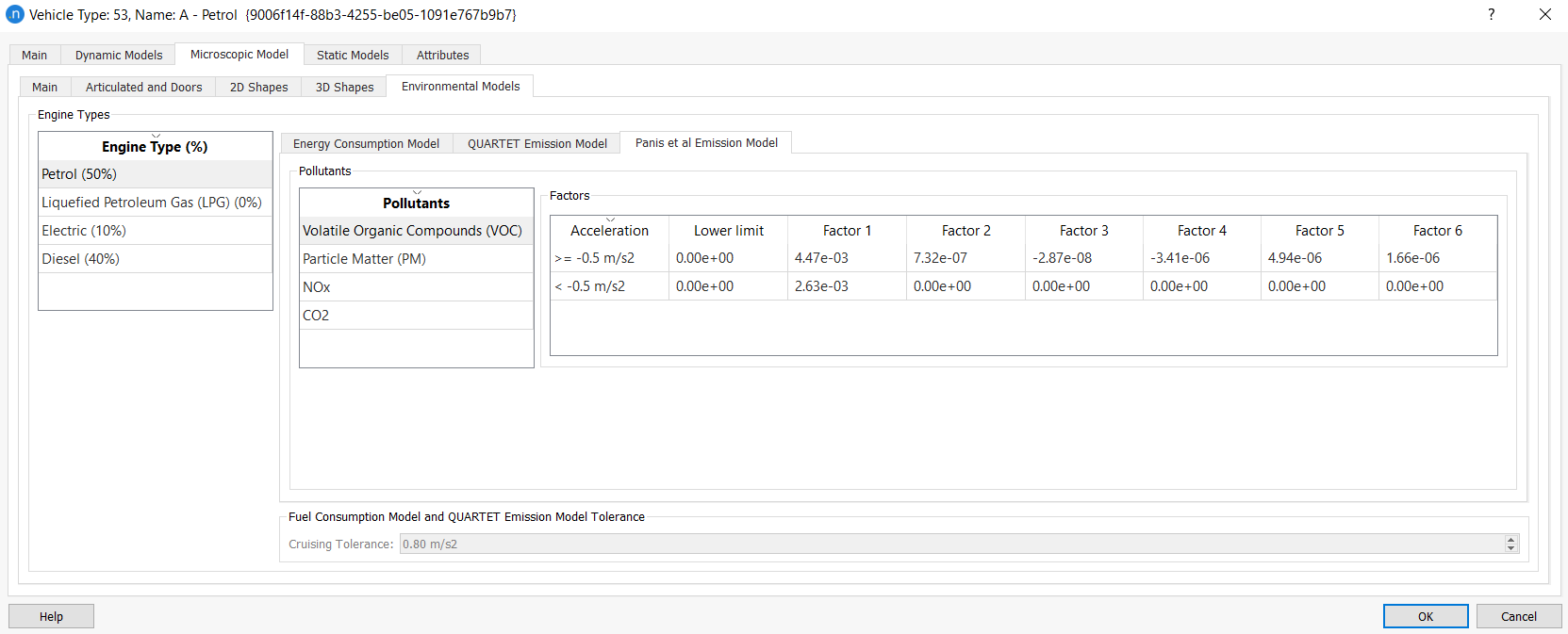
Note: The Panis Pollutant Emission Model assumes that Bus and HDV vehicles use Diesel. If the percentage in Petrol or LPG is greater than 0, the model will still only calculate pollution values for Diesel vehicles.

London Emission Model (LEM)

You can set the parameters for the LEM on the Vehicle Type dialog > Dynamic Models > London Emissions subtab. It is compatible with both microscopic and mesoscopic models.

Here you can define the emissions characteristics for each vehicle type, which will be used to allocate Euro emissions classes, by engine type, to each vehicle. This is according to the Emission Vehicle Type you select and the proportions set in the Engine Type (%) list.

These settings define how the emissions are estimated, using the LEM developed by ITS Leeds in collaboration with Transport for London and Aimsun.

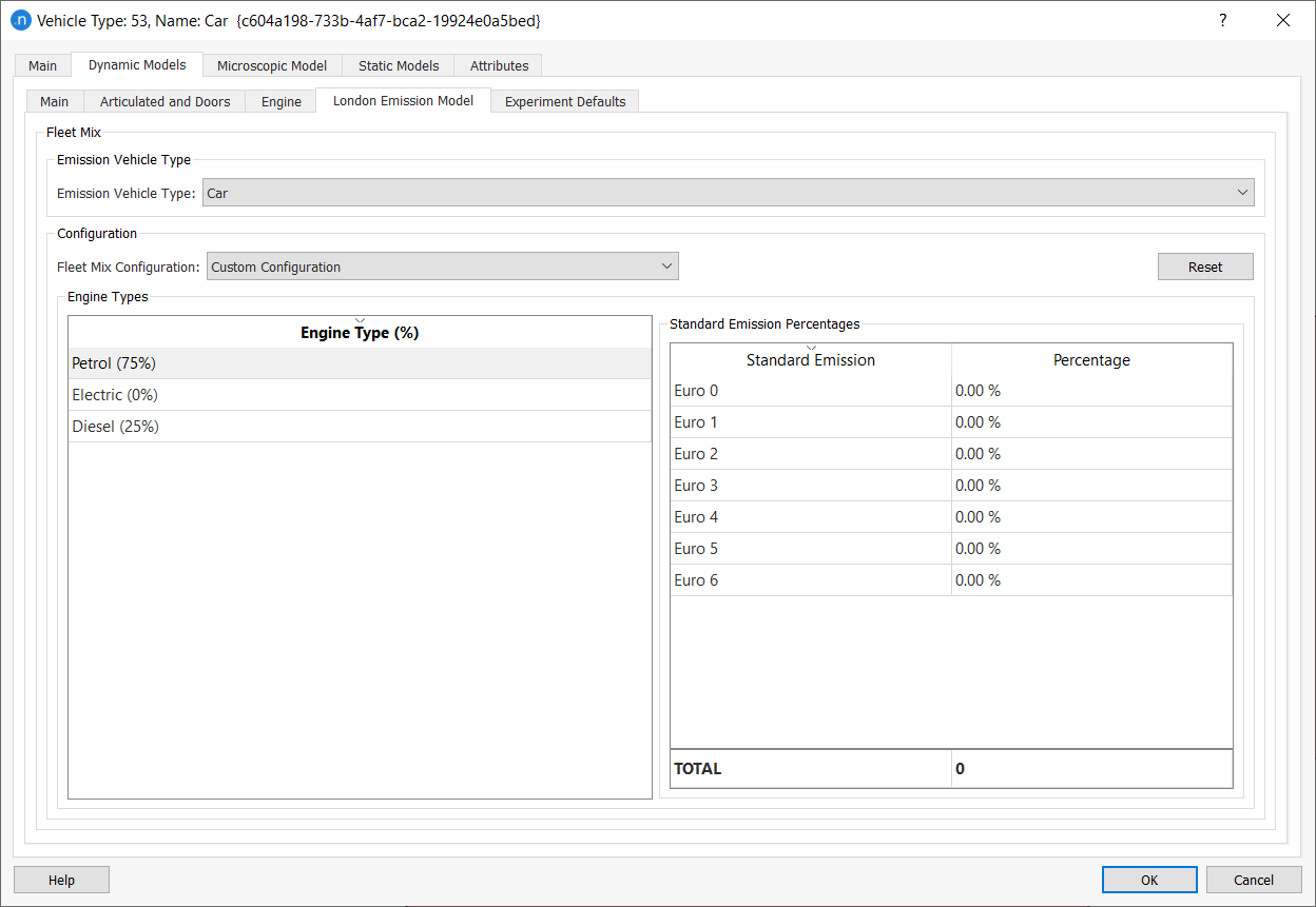
You can use the Emission Vehicle Type drop-down list to choose the class of vehicle you want to use in the emissions model, along with any subtypes supported by the vehicle category selected on the Engine tab.

The list contains Car and Taxi for the Car category, Large Goods Vehicle (LGV) and Heavy Goods Vehicle (LGV) for the Commercial vehicle category, and Single-Decker Bus, Double-Decker Bus, and Coach for the Bus category. These items are linked to calibrated values derived from measurements made when the model was developed.

You can set the fleet configuration for the selected vehicle type from the Fleet Mix Configuration drop-down list. The list includes available default configurations described by a location and a year (e.g. London 2017).

If you select Custom Configuration from the list, you can then edit the percentages for the Euro Emission Standard. Click Reset to change all values to zero.

For more information on the London Emission Model (LEM), refer to the London Emission Model chapter.

Static Models

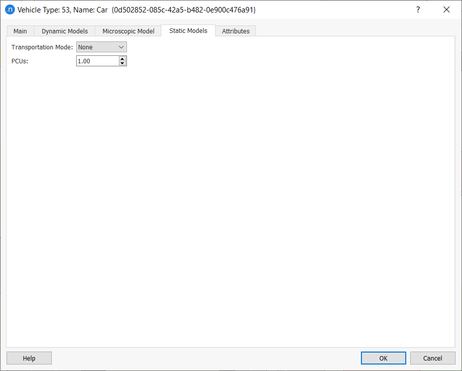
In the Static Models tab, two parameters are defined: Transportation Mode and PCUs.

• A Vehicle Type can belong to a Transportation Mode (for example, Car can belong to Mode Private). This information is used when modeling the Travel Demand with the Four-step Model.

• The PCUs parameter (Passenger Car Unit) is a measure of the space a Type of Vehicle needs compared to a passenger car. That is, the private car is considered as the unit, 1 PCU, and the rest of vehicles are converted to this unit by a factor.

Attributes

The attributes that characterize a vehicle type are set in this tab.