Environmental Models

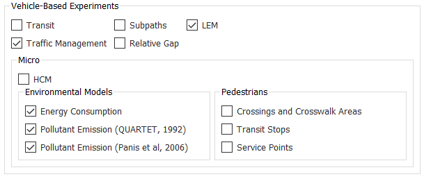
Aimsun Next microsimulation offers five environmental models: the Fuel Consumption Model, the Battery Consumption Model, the QUARTET Pollutant Emission Model, the Panis et al.'s Pollutant Emission Model, and the London Emissions Model (LEM). You can activate or deactivate each in the Scenario dialog on the Outputs to Generate > Statistics subtab (see below).

To activate the Battery Consumption Model and Fuel Consumption Model, you first need to tick Energy Consumption in the Environmental Models group box.

All the environmental models work according to engine type. The engine type composition for an Aimsun Next vehicle type can be set on the Vehicle Type dialog > Dynamic Models > Engine subtab. The Vehicle Type dialog also includes settings for Engine Type on the Dynamic Models > London Emission Model subtab and on the Microscopic Models > Environmental Models subtab.

The environmental models are available for petrol, diesel, and LPG engine types, with the exception of the Battery Consumption Model, which is only available for electric vehicles. Non-motorized vehicles are not included in any of the environmental models. Note: The only environmental models that include motorbikes are the Fuel Consumption Model and QUARTET Model.

The following sections explain how these models work, describing their input requirements and the outputs generated.

Note: Units in environmental models are metric.

Fuel Consumption Model

The Fuel Consumption Model only applies to combustion engine vehicles (petrol, diesel or LPG). It assumes that each vehicle is idling, cruising at a constant speed, accelerating, or decelerating. The state of each vehicle is determined by the simulator each time-step and the model then uses the appropriate formula to calculate the fuel consumed for the determined state.

For idling and decelerating vehicles, the rate (in ml/s) can be assumed to be constant. For an accelerating vehicle, it is given by the formula:

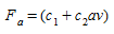
where \(c_1\) and \(c_2\) are constants and a and v are acceleration and velocity respectively.

The following fuel-consumption equation for a cruising vehicle moving at speed \(v\), has been determined by Akcelic 1982. It contains three constants: \(k_1\), \(k_2\), and \(v_m\), which need to be determined empirically for each vehicle type.

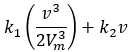
\(v_m\) is the speed at which the fuel consumed per km is at a minimum. Typically, this is approximately 50 km/h.

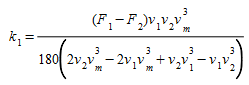
The UK Department of Transport 1994 provides fuel-consumption figures for all new cars. Among the figures given are the fuel consumption in liters per 100 km, for vehicles traveling at speeds of 90 km/h and 120 km/h. These figures can be used to determine the constants \(k_1\), \(k_2\) above.

It is easy to show that if \(F_1\) and \(F_2\) are the fuel-consumption rates in liters per 100 km/h for a vehicle traveling at a constant speed of either \(v_1\), \(v_2\) respectively, the equations are:

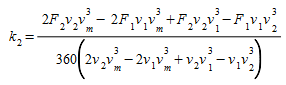
For each time step in the simulation, the state of each vehicle will be determined as either idling, accelerating, cruising at speed, or decelerating. The fuel consumed during the simulation time step, \(t\), will then be calculated for each vehicle according to its state using the formulae given in the table below, where \(F_i\) and \(F_d\) are the fuel-consumption rate in ml/s for idling and decelerating vehicles respectively and constants and need to be calibrated.

Vehicle state	fuel consumed (ml) during t
Idling	\(F_i\) Δ \(t\)
Accelerating with acceleration of \(a\) (m/s/s) and speed \(v\) (m/s)	(\(c_1\) + \(c_2av\)) Δ \(t\)
Cruising at speed \(v\) (m/s)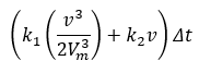
Decelerating	\(F_d\) Δ \(t\)

Input Parameters

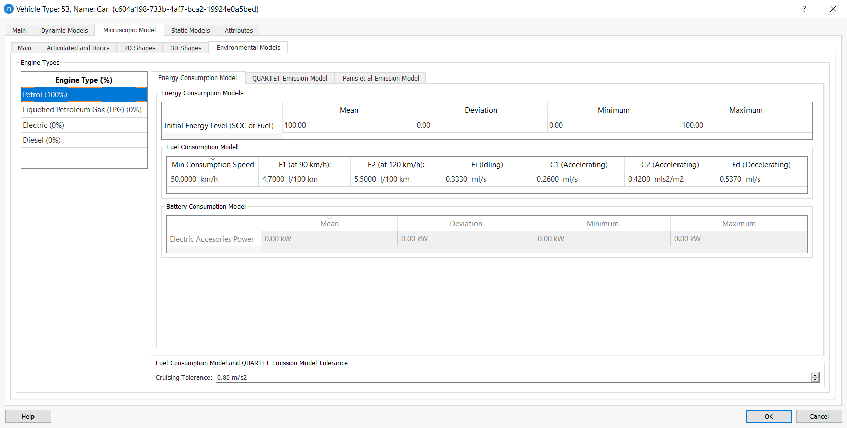
All the particular settings of the Fuel Consumption model can be found in the Energy Consumption subtab of the combustion engine types. For each vehicle type, the following additional six parameters specify the vehicle’s fuel-consumption rates, and need to be specified in the Vehicle Type dialog on the Microscopic Model > Environmental Models subtab:

• \(F_i\): The fuel-consumption rate for idling vehicles in ml/s.

• \(C_1\) and \(C_2\) : The two constants in the equation for the fuel-consumption rate for accelerating vehicles, in ml/s and in ml s²/m².

• \(F_1\): The fuel-consumption rate, in liters per 100 km, for vehicles traveling at a constant speed of 90 km/h.

• \(F_2\): The fuel-consumption rate, in liters per 100 km, for vehicles traveling at a constant speed of 120 km/h .

• \(F_d\): The fuel-consumption rate for decelerating vehicles in ml/s.

• \(V_m\): The speed at which the fuel-consumption rate, in ml/s, is at a minimum for a vehicle cruising at constant speed.

The following are example values of these input parameters, taken from Ferreira 1982 and the UK Department of Transport 1994.

The reference values in the study are only calibrated for vehicles: The fuel-consumption rate for idling vehicles (Fi) is 0.333 ml/s, and in the equation for the fuel-consumption rates for accelerating vehicles (C1;C2) are 0.420 ml/s and 0.260 ml s²/m². The fuel-consumption rate for decelerating vehicles (Fd) is 0.537 ml/s. The fuel-consumption rates for cruising vehicles are as follows:

Mini/Small Car (A/B):

\(F_1\) = 4.7 (1/100km at 90 km/h)

\(F_2\) = 5.5 (l/100km at 120 km/h)

\(V_m\) = 50 km/h

Medium/Large Car (C/D):

\(F_1\) = 5.4 (l/100km at 90 km/h)

\(F_2\) = 6.5 (l/100km at 120 km/h)

\(V_m\) = 60 km/h

Executive/Sport Utility Cars (E/F/J):

\(F_1\) = 6.4 (l/100km at 90 km/h)

\(F_2\) = 8.4 (l/100km at 120 km/h)

\(V_m\) = 70 km/h

Multi Purpose Cars/Cargo vans/Small passanger vans (M):

\(F_1\) = 7 (l/100km at 90 km/h)

\(F_2\) = 11.5 (l/100km at 120 km/h)

\(V_m\) = 50 km/h

Buses:

\(F_1\) = 25.0 (l/100km at 90 km/h)

\(F_2\) = 22.0 (l/100km at 120 km/h)

\(V_m\) = 40 km/h

Trucks:

\(F_1\) = 15–25 (l/100km at 90 km/h)

\(F_2\) = 16–24 (l/100km at 120 km/h)

\(V_m\) = 50 km/h

Motorbikes:

\(F_1\) = 2.8–4.8 (1/100km at 90 km/h)

\(F_2\) = 3.2–5.7 (l/100km at 120 km/h)

\(V_m\) = 50 km/h

We also included cruising values for buses and trucks, but please note that the other rates should be collected from the current literature.

Outputs

Outputs produced by the Fuel Consumption Model at the different levels of aggregation are as follows:

• For the entire network, the total distance traveled (in km) by all vehicles that have finished their trip, and the total fuel consumed by them, in liters.

• For each section and turn, the kilometers traveled by all vehicles that have crossed the section, and the total fuel consumed by them, in liters.

• For each route, the total distance traveled (in km) by all the vehicles that have followed the route, and the total fuel consumed by them, in liters.

Battery Consumption Model

The Battery Consumption Model only applies to electric vehicles. It is based on the following paper:

Fiori, C., Ahn, K., & Rakha, H. A. (2016). Power-based electric vehicle energy consumption model: Model development and validation. Applied Energy, 168, 257-268.

The model was set up using publicly available data for Nissan Leaf. However, the model included in Aimsun Next has been extended to cover other vehicle types, following the same vehicle profiles (by Euro Car Segments) in the MFC acceleration model.

The only vehicle type currently supported is Car and Aimsun Next adheres to the Euro Car Segments: A, B, C, D, E, F, J, and M. The model depends on vehicle dynamics, meaning that the MFC model must be activated first in order for the Battery Consumption Model to be applied to electric vehicles.

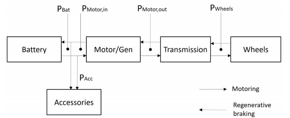
The Battery Consumption Model uses a backward-looking approach: from the vehicle speed cycle to the engine dynamics by means of the MFC acceleration model. In this way it obtains the motor/generator power train of the engine to get the instant state of charge (SOC).

It also considers the efficiency of the different processes involved in the operation of the vehicle: the motor/generator, regenerative braking, and transmission, as described in the paper.

The implemented model includes an extension of Fiori's et al. model to capture the effect of the ambient temperature (in the range of −15°C to 20°C), due to the consequent accessory power required for heating (or cooling) the vehicle's cabin, which is described in the following paper:

Iora, Paolo & Tribioli, Laura. (2019). Effect of Ambient Temperature on Electric Vehicles’ Energy Consumption and Range: Model Definition and Sensitivity Analysis Based on Nissan Leaf Data. World Electr. Veh. J. 2019, 10(1), 2..

The model is represented by the diagram below. There are two modes of vehicle operation: motoring, where the engine is used as a motor (battery energy flows to power the wheels) and regenerative braking, where the engine is used as a generator (energy recovered from the brakes flows to the battery). The image illustrates both modes at work.

Inputs

You can find all the particular settings of the Battery Consumption Model on the Vehicle Type dialog > Microscopic Model > Environmental Models > Energy Consumption Model subtab.

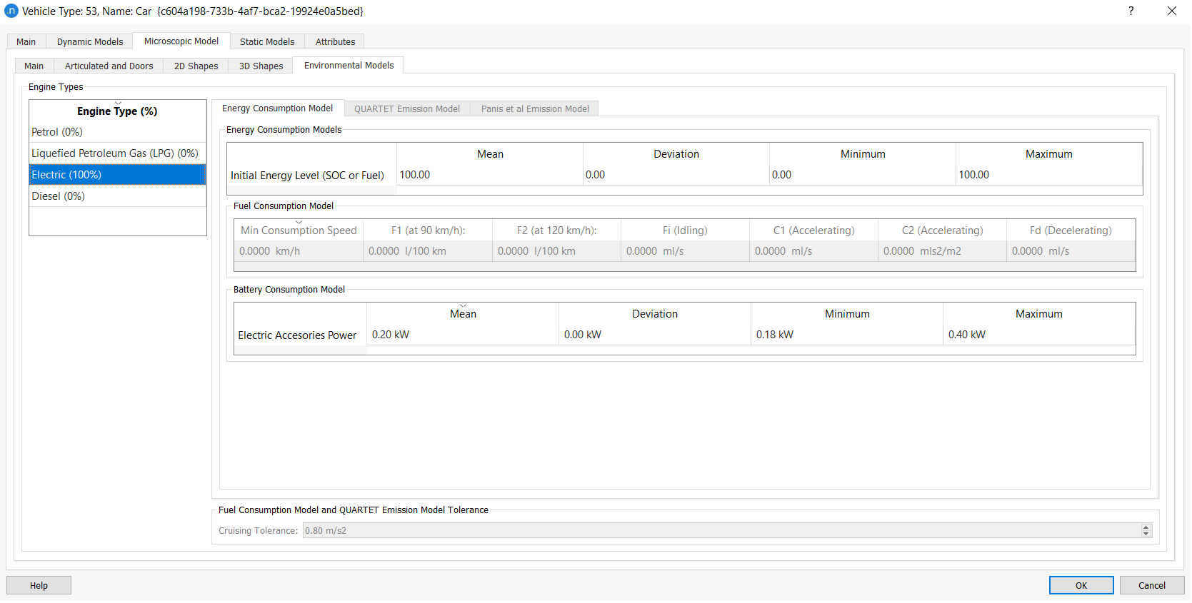
Because this model depends heavily on the parameters of the MFC acceleration model – specified at the level of vehicle type – the vehicle category and the composition of the engine type are crucial choices when running this model.

The Vehicle Type dialog also includes a parameter for the Initial Energy Level (SOC or Fuel) of each vehicle, using normal distribution, as is the case with other vehicle type parameters. You can directly edit the values for Mean, Deviation, Minimum, and Maximum.

Outputs

The outputs produced by the Battery Consumption Model at different levels of aggregation are as follows:

• For the entire network, the total distance traveled (km) by all vehicles that have finished their trip, and the total amount of battery consumed by them (kWh).

• For each section and turn, the kilometers traveled by all vehicles that have crossed the section, turn, or link, and the total battery consumed by them (kWh).

• For each route, the total distance traveled (km) by all the vehicles that have followed the route, and the total amount of battery consumed by them (kWh).

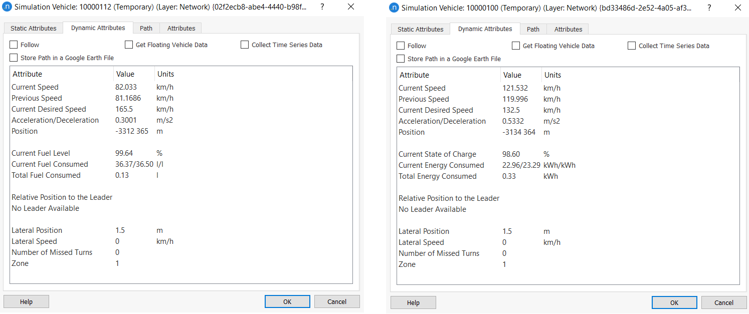
When using an energy consumption model for a vehicle, the Simulation Vehicle dialog displays the following attributes on the Dynamic Attributes tab:

• Current Fuel State/Current State of Charge
• Current Fuel Level/Current Energy Level
• Total Fuel Consumed/Total Energy Consumed.

QUARTET Pollutant Emission Model

Aimsun Next can model pollutant emissions for all vehicles in the simulation. As in the Fuel Consumption Model, the vehicle state (idling, cruising, accelerating, or decelerating) and the vehicle speed/acceleration is used to evaluate the emission from each vehicle for each simulation time step.

This is done by referencing look-up tables for each pollutant, which give emissions (in g/s) for every relevant combination of vehicle behavior, and speed/acceleration. There are different sets of look-up tables for each vehicle type and each pollutant.

Currently, a maximum of three pollutants are considered, corresponding to the three most widely produced pollutants (carbon monoxide, nitrogen oxides and unburned hydrocarbons) but we might be able to model additional pollutants when and if extra data becomes available.

Input Parameters

The inputs required for the QUARTET Pollutant Emission Model are the following:

• For each vehicle type (e.g. cars, buses, trucks)

  • For each pollutant modeled (i.e. CO, NO_x, HC)

    • Name of the pollutant

    • Emission rate for accelerating vehicles in g/s (AER parameter in the dialog)

    • Emission rate for decelerating vehicles in g/s (DER parameter in the dialog)

    • Emission rate for idling vehicles in g/s (IER parameter in the dialog)

    • A look-up table for vehicles cruising at a constant speed, consisting of a set of pairs (speed break point (km/h), emission rate (g/s)) for a maximum of 15 break points.

    • A look-up table for the slope impact on the pollution consisting of a set of triples (speed break point (km/h), Slope %, Impact). Depending on the vehicle speed and slope %, the pollution will be multiplied by the impact.

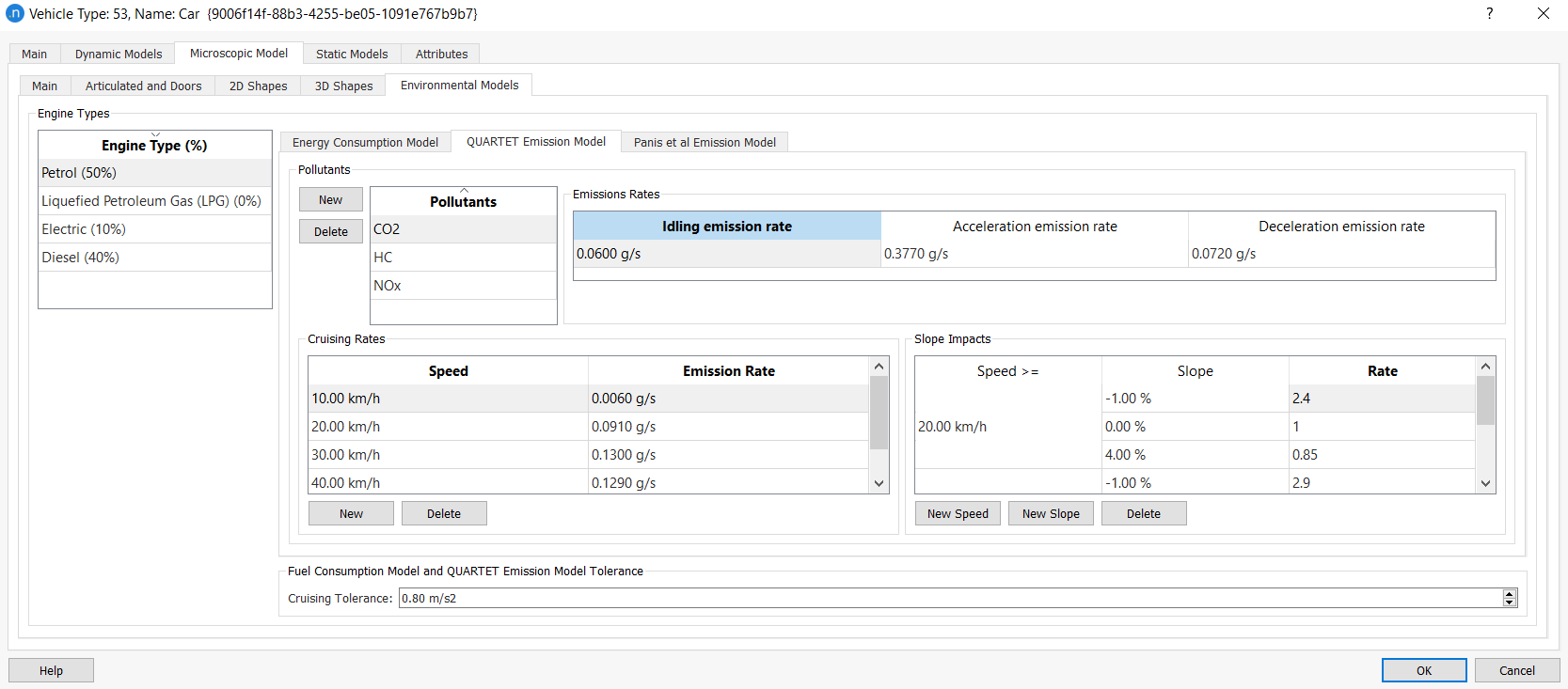
Emission values for petrol cars and buses, taken from a QUARTET deliverable in 1992, are summarized in the next two tables.

Emission rates for cars (g/s)	CO	NOx	HC
Idling emission rate (g/s)	0.060	0.0008	0.0067
Accelerating emission rate (g/s)	0.377	0.0100	0.0200
Decelerating emission rate (g/s)	0.072	0.0005	0.0067
Cruising emission rate (g/s)
10 km/h	0.060	0.0006	0.0063
20 km/h	0.091	0.0006	0.0078
30 km/h	0.130	0.0017	0.0083
40 km/h	0.129	0.0022	0.0128
50 km/h	0.090	0.0042	0.0097
60 km/h	0.110	0.0050	0.0117
70 km/h	0.177	0.0058	0.0136

Emission rates for buses (g/s)	CO	NOx	HC
Idling emission rate (g/s)	0.050	0.0050	0.0383
Accelerating emission rate (g/s)	0.377	0.0100	0.0200
Decelerating emission rate (g/s)	0.072	0.0005	0.0067
Cruising emission rate (g/s)
10 km/h	0.097	0.018	0.078
20 km/h	0.056	0.020	0.044
30 km/h	0.050	0.023	0.042
40 km/h	0.069	0.036	0.056
50 km/h	0.056	0.067	0.078
60 km/h	0.042	0.083	0.067
70 km/h	0.000	0.133	0.067

Outputs

Output produced by the QUARTET Pollutant Emission Model at the different levels of aggregation are as follows:

• For the entire network, the total distance traveled (in km) by all vehicles that have finished their trip, and the kilograms of each pollutant emitted by them.

• For each section and turn, the total distanced traveled (in km) by all vehicles that have crossed that section, and the kilograms of each pollutant emitted by them.

• For each route, the total distance traveled (in km) by all vehicles that have followed that route, and the kilograms of each pollutant emitted by them all.

Panis et al. Pollutant Emission Model

Aimsun Next can model instantaneous pollution emissions caused by acceleration/deceleration and speed for all the vehicles in this model of simulation. It is based on the paper by Luc Int Panis, Steven Broekx, and Ronghui Lui: Modelling instantaneous traffic emission and the influence of traffic speed limits.

At each simulation time step this model measures the emissions for each pollutant using the same formula. However, it considers different values of factor according to the vehicle type, the fuel type, and instant acceleration/deceleration measures.

In particular, the instantaneous emission model considers carbon dioxide (CO₂), nitrogen oxides (NO_x), volatile organic compounds (VOC), and particulate matter (PM).

Input Parameters

Each vehicle type included in the simulation must have its instantaneous emissions parameters defined. You can do this in the Vehicle Type dialog on the Microscopic Model > Environmental Models subtab.

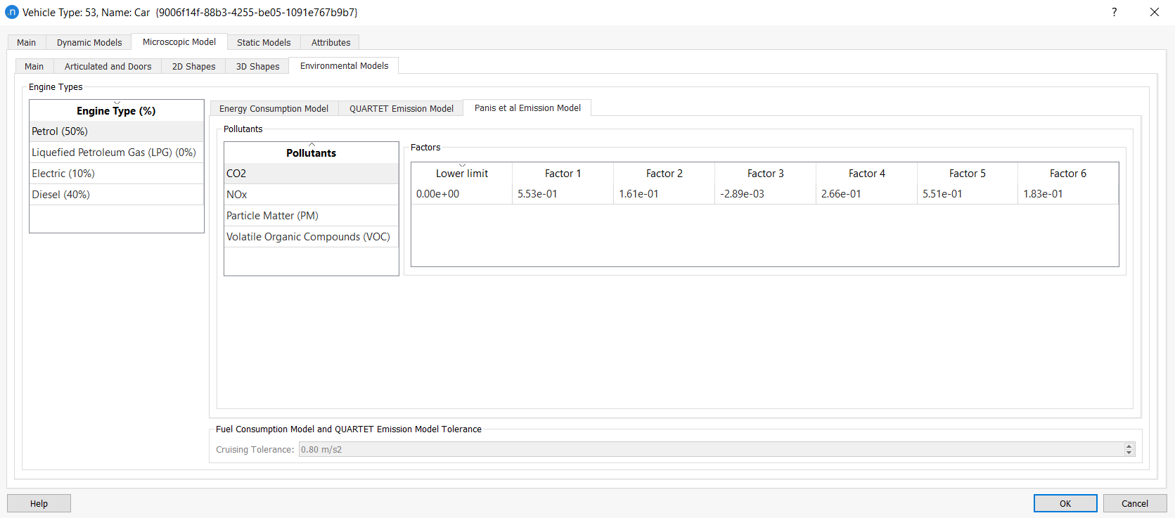
Note that the model assumes that the vehicle type Car can use Petrol, Diesel, LPG (liquefied petroleum gas) or EV (electric). By default, 75% Diesel and 25% Petrol are assumed at first. Bus and HDV vehicles can use Diesel or EV but, by default, only diesel is assumed. Also, the model does not include the calculation of PMs in the case of EV, considering the value to be zero.

Outputs

When the simulation is complete, eight time series will be added to the sections, nodes, turns, and the replication. There will be two for each kind of pollutant (CO₂, NO_x, VOC, and PM), giving their values in g and in g/km (labeled as "interurban"). Time series can be viewed in each affected object's dialog, on the Time Series tab.

If you ticked Statistics: Store in Database on the Outputs to Generate tab of the scenario, these seven tables will appear in the selected database: MISYSIEM, MISECTIEM, MITURNIEM, MINODEIEM, MISTREAMIEM, MIPTIEM, and MIODPAIRIEM. For more information about such tables, see Output Database Definition.

London Emission Model (LEM)

The London Emission Model (LEM) is included in the Aimsun Next microscopic, mesoscopic, and hybrid simulators. This estimates the CO₂ and NO_x emissions for a vehicle, using a calibrated average speed emissions model developed in collaboration with Transport for London (TfL) in 2017.

The LEM was developed as a model which could take into account the variability in vehicle activity and give more accurate emissions on short links or for short time periods than traditional average speed models.

The LEM derives the emissions for a vehicle using the average speed for a particular vehicle type. The instantaneous model PHEM was applied to a set of real world drive cycles measured in London 2017. These measurements were then generalized to give a relationship between average speed and emissions. The approach taken by the LEM model was to derive the emissions for an individual vehicle using its average speed over a set of micro-trips which make up its journey

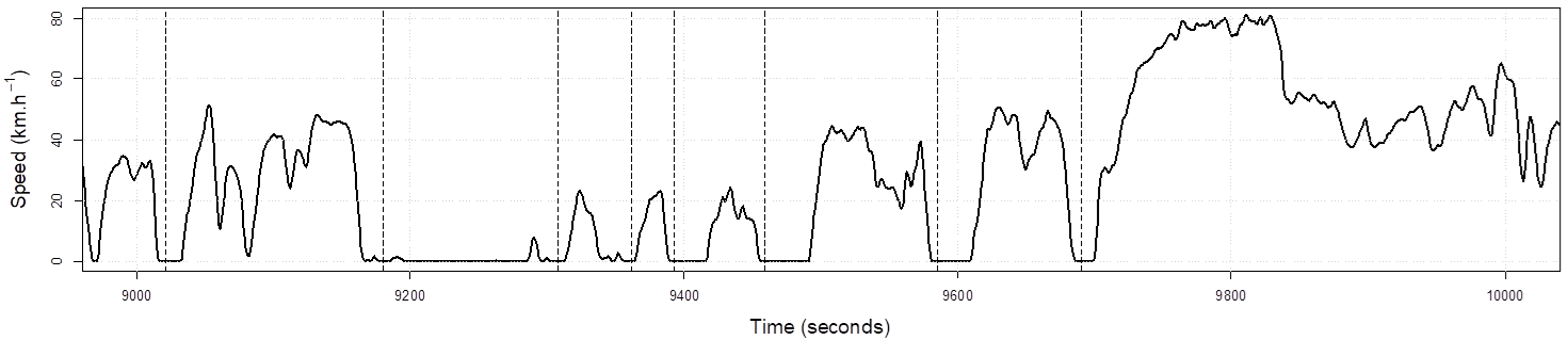
A micro-trip is defined as a segment of a trip where the speed rises from stationary to > 5 km/h and back to stationary. This is illustrated below in a typical plot of speed vs time in an urban drive cycle.

The LEM then uses one of two polynomial relationships, derived by regression analysis, to estimate the CO₂ and NO_x produced by that vehicle using that micro-trip.

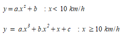
Here, y is the emission (grams/km); a, b, c, and z are derived constants which are defined for each vehicle and euro type, x is the average speed in the micro-trip.

Within Aimsun Next, the average speed of an individual vehicle within a section or a link are used to then derive the emissions of that vehicle locally. The total emissions for the network is taken to be the sum of the emissions of all vehicles on all sections.

It is important to note when using this model that it is calibrated for urban and city conditions and should not be used for highways which can have different drive cycles.

Input Parameters

The proportion of vehicles of a particular fuel type and Euro class is defined in the vehicle type on the London Emissions Model > Fleet Mix Tab.

The model considers the following fuel types and Euro classes:

Emission Vehicle Types	Fuel Types	Standard Emissions
Car	Petrol	Euro 0, Euro 1, Euro 2, Euro 3, Euro 4, Euro 5, Euro 6
	Diesel	Euro 0, Euro 1, Euro 2, Euro 3, Euro 4, Euro 5, Euro 6, Euro 6c
	Electric	Zero emissions
Taxi (London Taxi)*	London Taxi Fuel	Euro 0, Euro 1, Euro 2, Euro 3, Euro 4, Euro 5, Euro 6
	Electric	Zero emissions
Large Goods Vehicle (LGV)	Petrol	Euro 0, Euro I, Euro II, Euro III, Euro IV, Euro V, Euro VI
	Diesel	Euro 0, Euro I, Euro II, Euro III, Euro IV, Euro V, Euro VI
	Electric	Zero emissions
Heavy Goods Vehicle (HGV)	Diesel	Euro 0, Euro I, Euro II, Euro III, Euro IV EGR, Euro V EGR, Euro V SCR, Euro VI
	Electric	Zero emissions
Single-Decker Bus	Diesel	Euro 0, Euro I, Euro II, Euro III, Euro IV, Euro V EGR, Euro V SCR, Euro VI
	Electric	Zero emissions
Double-Decker Bus	Diesel	Euro 0, Euro I, Euro II, Euro III, Euro IV, Euro V EGR, Euro V SCR, Euro VI
	Electric	Zero emissions
Coach	Diesel	Euro 0, Euro I, Euro II, Euro III, Euro IV, Euro V EGR, Euro V SCR, Euro VI
	Electric	Zero emissions

Note: The taxi defined in the LEM is for the London Hackney Taxi and which would not include private hire vehicles (PHVs). For private hire vehicles it is recommended to use the generic LEM vehicle type, car.

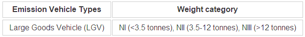
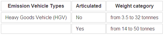
The model does not take the gradient of roads into account. However, the model does take into account the weight of the vehicle within Aimsun Next to define more detailed a, b, c, and z constants for large goods vehicles and heavy goods vehicles. If the vehicle type uses the HGV type within the London Emissions model, it can also be considered to be articulated when over a certain weight. This is defined as below.

You can activate or deactivate the model's outputs in the Scenario dialog on the Outputs to Generate > Statistics subtab.

Outputs

You can activate or deactivate the model’s outputs in the Scenario dialog on the Outputs to Generate > Statistics subtab.

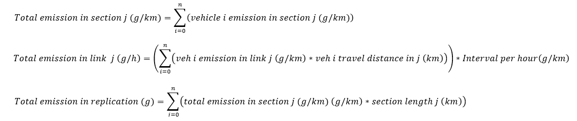
When the simulation is complete, two time series for CO₂ and NO_x will be added to the sections (g/km), links (g/h), and the replication (g). Time series can be viewed in each affected object’s dialog, on the Time Series tab.

If you ticked Statistics: Store in Database on the Outputs to Generate tab of the scenario, three tables will be added to the selected database: SECTLEM, LINKLEM, and SYSLEM. For more information on these tables, see Output Database Definition.