Dynamic User Equilibrium (DUE)

For a DTA to become a DUE the behavioral assumptions on how travelers choose the routes have to be consistent with the dynamic user equilibrium principle. Ran and Boyce 1996, formulate the dynamic version of Wardrop’s user equilibrium in the following terms: If, for each OD pair at each instant of time, the actual travel times experienced by travelers departing at the same time are equal and minimal, the dynamic traffic flow over the network is in a travel-time-based dynamic user equilibrium (DUE) state.

Heuristic approach in Aimsun Next

This formulation could correspond to the hypothetical scenarios on which ATMS and ATIS application will work and reliable traffic information/traffic prediction systems will become available to travelers, allowing them to adjust their behaviors accordingly. Alternatively it can be considered as the realization of a process in which travelers adjust their current information with conjectures about the expected traffic conditions ahead; this could correspond to the process followed by commuters adapting their behavior according to a day-to-day learning process depending on the fluctuations of traffic patterns until they consider that no further improvement is possible. This interpretation is implemented in a microsimulation approach by an iterative heuristic procedure that mimics the day-to-day learning process leading to a solution that can be interpreted as a DUE, Barcelo and Casas 2002, Liu et al. 2005.

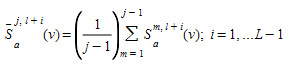
The implementation in Aimsun Next replicates the simulation N times and link costs for each link j, for each time interval t, t+1, ..., L (where L = T/t, T being the simulation horizon and t the user-defined time interval in which to update paths and path flows) at every iteration n are stored. Thus at iteration n the link costs of previous iteration n-1 can be used to estimate the expected link cost at the current iteration. Let S~a~^jl^(v) be the current cost of link a with flow v, at iteration l of replication j, then the average link costs for the future L-l time intervals, based on the experienced link costs for the previous j-1 replications is given by

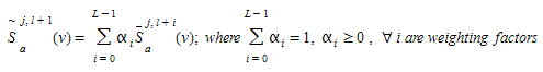
The “forecasted” link cost can then be computed as:

The resulting cost of path k for the i-th OD pair is given by:

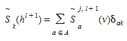
where, as usually the arc-path incidence matrix δ~ak~ is:1 if link a belongs to path k and 0 otherwise.

The path costs are the arguments of the route choice function (logit, C-logit, proportional, user defined, etc.) used at iteration l+1 to split the demand g~i~^l+1^ among the available paths for OD pair i.

The default implementation in the current version of Aimsun Next uses a simplified version consisting of a link cost function defined as:

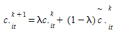
Where c~it~^k+1^ is the cost using link i at time t at iteration k+1, and c~it~^k^ and c\~~it~^k^ correspond respectively to the expected and experienced link costs at this time interval from previous iterations.

Algorithmic approaches for DUE

It can be shown that the DUE approach can be implemented in terms of solving the following mathematical model:

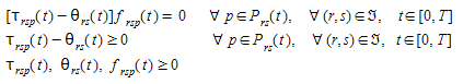
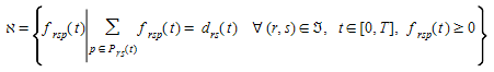
And the flow balancing equations

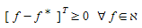
Where, as before, f~rsp~(t) is the flow on path p from r to s departing origin r at time interval t, τ~rsp~(t) is actual path cost from r to s on route p at time interval t, θ~rs~(t) is the cost of the shortest path from r to s departing from origin r at time interval t, P~rs~(t) is the set of all available paths from r to s at time interval t, is the set of all origin-destination pair (r,s) in the network and d~rs~(t) is the demand (number of trips) from r to s at time interval t. It can be shown that this is equivalent to solve a finite dimensional variational inequality problem consisting on finding a vector of path flows f* such that:

Wu et al. 1991, Wu et al. 1998a and 1998b, prove that this is equivalent to solve the discretized variational inequality:

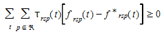
Where is the set of all available paths. A variety of algorithms have been proposed to solve this variational inequality from projection algorithms: (Wu et al 1991, Wu et al. 1998a, Wu et al. 1998b, Florian et al. 2001) or methods of alternating directions, Lo and Szeto 2002, to various versions of the Method of Successive Averages (MSA), Tong and Wong 2000, Varia and Dhingra 2004, Florian et al 2002, Mahut et al. 2003a, Mahut et al. 2003b, and Mahut et al. 2004. The MSA procedure redistributes the flows among the available paths in an iterative procedure that at iteration n computes a new shortest path from origin r to destination s at time interval t, c~rs~(t), then the paths flows update process is:

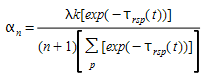
Depending on the values of the weighting coefficients αn, different MSA schemes can be implemented Carey and Ge 2007. Perhaps the most typical value is:

An interesting modified MSA algorithm is described in Varia and Dhingra 2004, where the weighting coefficient takes into account a variable step length which depends on the current path travel times:

One of the potential computational drawbacks of these implementations of MSA is the growing number of paths in the case of large networks; to avoid this in the case of the DTA assignments in Aimsun Next the user has the option to specify the maximum number K of paths to keep for each origin-destination pair, therefore in implementing the MSA in Aimsun Next, it was considered that it would be desirable to keep this feature.

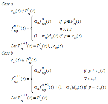
Several modified MSA implementation have been proposed to keep control on the number of paths in MSA algorithms, Peeta and Mahmassani 1995, Sbayti et al. 2007, however, possibly one of the most efficient computationally is the one proposed by Florian et al. 2002 (see also Mahut et al. 2003b and 2004) modifying the MSA algorithm to keep bounded the number of alternative paths to account for each origin-destination pair. This variant of the algorithm initializes the process on basis to an incremental loading scheme distributing the demand among the available shortest paths, the process is repeated for a predetermined number of iterations after which no new paths are added and the corresponding fraction of the demand is redistributed according to the MSA scheme. The modified MSA works as follows:

Let K be the maximum number of iterations to compute new paths:

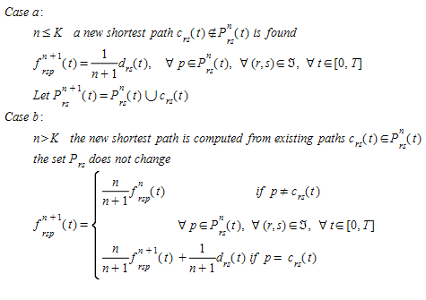
This is the version of the MSA algorithm implemented in Aimsun Next. However, taking into account the possibility of repeating shortest paths from one iteration to the next to keep a maximum of K different shortest paths a proper implementation of the algorithm requires that the number of iterations n is defined by OD pair and time interval.

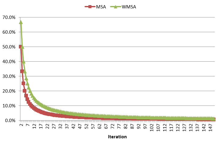
In Aimsun Next, a modification of MSA algorithm is available named WMSA proposed by Liu et all 2007. The MSA algorithm in iteration n, 1/n of the demand is moved, and in WMSA 2/(n+1) of the demand is moved.The next figure shows the amount of demand moved as a function of iteration number.

The convergence criterion

All the proposed approaches for DUE are based on simulation procedures for the network loading process and therefore are heuristic in nature, so no formal proof of convergence can be provided. Consequently, a way of empirically determining whether the solution reached can be interpreted in terms of a DUE, in the sense that “the actual travel time experienced by travelers departing at the same time are equal and minimal” can be based on an ad hoc version of the Relative Gap function proposed by Janson 1991:

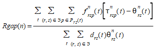
Where

• f~rsp~^n^(t) is the flow on path p departing from origin r at time t at iteration n with destination s.
• τ~rsp~^n^(t) is the experienced or instantaneous cost of path p.
• θ~rs~^n^(t) is the shortest path cost for paths departing from origin r at time t at iteration n with destination s.

The difference τ~rsp~^n^(t) - θ~rs~^n^(t) measures the excess cost experienced by the fact of using a path p instead the shortest path.

In previous versions, the shortest path cost in the RGap formula for paths departing from origin θ~rs~^n^(t) was that of the path with the minimum cost among the set of used paths. From Aimsun Next 22, this is the cost of the newly calculated shortest path with the updated costs at the end of the iteration.

This is more accurate and allows a better assessment of the RGap for OD pairs in which all vehicles use the same path. However, you might observe that the RGap in Aimsun Next 22 is higher and that the DUE performs more iterations in order to converge. If this concerns you, you can still use the previous calculation by adding a new experiment variable with the name $DTARGAPEVALUATION and a value of RGAP20.

The ratio measures the total excess cost with respect to the total minimum cost if all travelers had used shortest paths.

As stopping criterion, a default global Relative Gap can be set in the Dynamic Traffic Assignment tab of the experiment editor for a specific number n of consecutive iterations (by default n = 1). A relative gap matrix with different thresholds can be set for each OD pair too. When a Relative Gap Matrix is defined, for those OD pairs with a value greater than 0, the local OD threshold is used, otherwise the DUE process uses the global relative gap.

In the DUE process with global relative gap, there is the possibility to include other two additional convergence criteria:

• A percentage x% of links with a flow change below y% for at least n consecutive iterations (by default n = 4).
• A percentage x% of links with a cost change below y% for at least n consecutive iterations (by default n = 4).

These two additional criteria are by default deactivated and can be activated individually from the Dynamic Traffic Assignment tab of the experiment editor. Once active, the convergence is achieved when both the gap criterion and the flow/cost criteria are fulfilled, or when the maximum number of iterations is achieved.

The computational framework in Aimsun Next

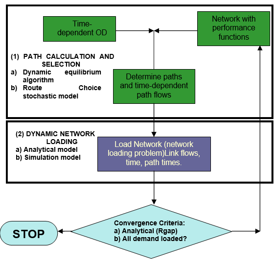
The computational framework for DTA proposed by Florian 2001 and Florian 2002 consists of two components:

1. A method to determining the path dependent flow rates on the paths on the network
2. A Dynamic Network Loading method, which determines how these path flows give raise to time-dependent arc volumes, arc travel times, and path travel times.

This has been implemented in Aimsun Next as shown in the conceptual diagram below. When the Dynamic Scenario dialog is selected, the system offers three options: microscopic, mesoscopic, and hybrid, which determine the simulation approach on which the network loading is based; and for each network loading, two alternatives are offered: DTA or DUE.

• DTA is based on the described heuristic approach using stochastic route choice models.
• DUE is based on the iterative heuristic described above and on the MSA or Gradient-based algorithms.

The convergence criteria depends on the alternative selected: the completion of the demand loading in the DTA and either the completion of the number of defined iterations or when the Rgap function reaches the desired accuracy.

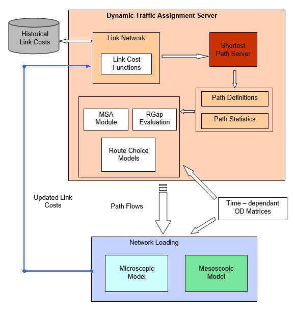
An efficient computational implementation of this conceptual approach requires that the analytical part of the process, that is the path calculation and selection is implemented independently of the dynamic network loading process selected to implement the heuristic part of the Dynamic Traffic Assignment. In other words when the network consistency holds for the meso and micro representation the path calculation based on time dependent link costs must be the same and the only difference will depend on the values of the arguments of the link cost functions that will be provided respectively by the mesoscopic traffic simulation or the microscopic traffic simulation used for the Dynamic Network Loading.

The integrated software architecture of Aimsun Next allows such common calculation of shortest paths given that network representations share the same object model and model database and vehicles can be unique and the same for meso and micro if the meso model is based on an approach that individualizes vehicles, then path calculation can be carried out by a common “shortest path server” and are the same at both levels. The conceptual approach for dynamic traffic assignment proposed in the previous figure has been implemented in terms of a “Dynamic Traffic Assignment Server”. The structure of this server is shown below.

DUE Parameters

Before running the model, the parameters of the Dynamic User Equilibrium are defined in the properties of the Experiment in Dynamic Traffic Assignment tab.

Estimation of path flow rates

The new approach implements the estimation of the path flow rates based on a Dynamic User Equilibrium (DUE). This process implements an iterative process to minimize the Relative Gap by applying the method of the successive averages (MSA),

Start and Continue a Dynamic User Equilibrium

Continuing or starting a DUE from a previous DUE or a Macro Assignment using an APA file is possible whether the network has been changed or not. The first iteration when starting or continuing a DUE using a previous assignment is used to calculate the link costs. If the network has been changed, The APA fixer can be used to ensure the network and the APA file are consistent. The APA fixer checks an APA file and corrects it based on the current network configuration. The APA fixer implements the following changes:

• Addition and removal of centroids and/or connectors
• Addition, removal or modification of turns and/or turn connection entity definitions
• Addition, removal or modification of sections

The APA fixer is a command line tool which takes as input:

• The original APA file
• The revised network
• The identifier for the experiment in revised network.

The new APA file is output to a new directory "correctedapa" located in the same directory as the original APA.

In the three cases the APA fixer assures that the resulting APA file will be compatible with the new network and will assure that the previous assignment is consistent. So for every origin and destination the assignment sums up to 100%.

Incremental Result

In order to improve the overall convergence process and get better routes an incremental result can be used. The difference between a normal result and an incremental result is the number of outer iterations. In a normal result there is only one outer iteration using the demand defined in the scenario. In an incremental result the user can specify a number of outer iterations with different increasing percentages. The percentage of each outer iteration defines the proportion of the demand that is going to be used. First iterations have lower demand and this demand is increased at each outer iteration with a 100% of the demand in the last iteration.

The goal is to develop routing in an uncongested network to avoid the distortion in routing bought on by over congestion in the simulation.