Transport Planning and Demand Analysis Models and Algorithms in Aimsun Next

The Four Step Model in Transport Planning

Urban travel demand and mobility analysis have evolved into a well-established methodology, commonly referred to as the four steps model.

This section describes the Transport Planning and Demand Analysis Models implemented in Aimsun Next and the algorithms they use. It is composed of the following sections:

• System Architecture
• Zones
• Network
• Trip Generation
• Trip Distribution
• Static Assignment
• Static Adjustment

System Architecture

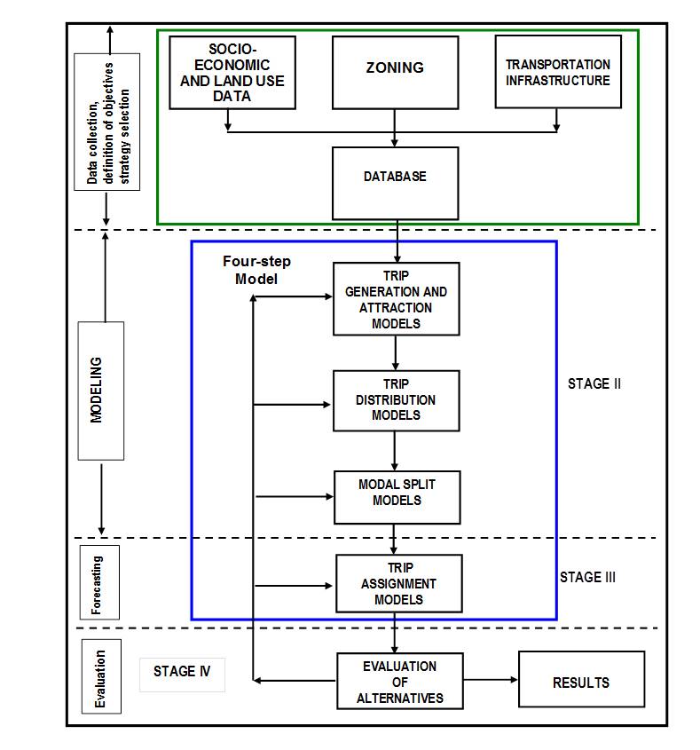
Ortúzar and Willumsen (2001), propose a general methodology conceptually depicted in the diagram below, which embeds the classical four steps model within it. Their methodological approach consists of the following stages:

• Stage I:

  The objectives of the study are defined, the strategies to achieve those objectives are selected, and the data necessary to conduct the study are collected. This usually implies:

  • The collection of the socioeconomic and land use data, usually structured according to a zoning scheme partitioning the area that is the object of the study.
  • The collection of all the information concerning the transportation infrastructure: motorways, highways, roads, streets and urban streets, transit lines, railways, etc.

• Stage II:

  This is the modeling stage, and contains three of the four steps of the four step model: - The construction of the Trip Generation and Attraction models (Step I) - The construction of the Trip Distribution models (Step II) - The construction of the Modal Split models (Step III)

• Stage III:

  The forecasting stage, also known as the Trip Assignment Models.This is Step IV of the four step transport model.

• Stage IV:

  The evaluation stage; the results of the forecast are analyzed and evaluated using the criteria identified in stage I. The results are reported and delivered to decision makers.

Process

The methodology, as represented in the diagram, with the Four Steps Model highlighted in the blue box, should be understood as an iterative process in which the results of any stage can lead to the re-evaluation of the previous ones, or a need for new data or evidence to refine the prior stages.

The modeling tools and algorithms in the transport planning and demand analysis components in Aimsun Next have been designed to support the transport analyst in applying the most relevant functions of the four step model.

Zones

Transportation analysis is conducted with models whose components are:

• The transportation infrastructure and services: i.e. the road network, transit, etc.
• The transportation system operation and control policies.
• The demand for travel including activity and land use patterns, i.e. the zone scheme.

Travel is an activity that takes place moving from one location to another over a transportation network (Oppenheim, 1995). Thus, most of the concepts used in modeling transport systems have a spatial dimension and the first question to be addressed is how represent the spatial structure.

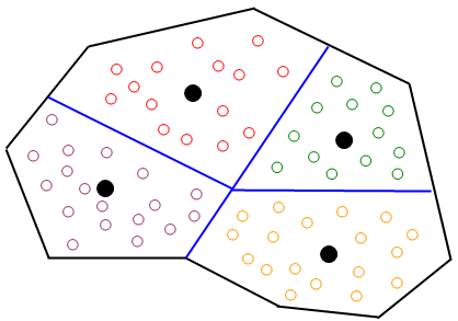
The traditional approach is to use a set of aggregated zones, in which traveler’s locations are bundled into “traffic zones” defined by the analyst. The size of each traffic zone can vary from a city block to a whole neighborhood or a town depending on the requirements of the model. Each traffic zone is represented by a “centroid” node (located usually at the geometrical or gravity center of the zone). The abstracted spatial structure corresponding to a given geographic structure can be visualized in a hypothetical area as in figure below, in which each white dot represents an individual traveler’s location and black dots the zone centroids. In the transportation planning process the typical representation of the demand consists of a partition of the area under study into traffic zones. The key to successful modeling is to determine the appropriate number and size of these zones.

Network

The transportation infrastructure is modeled in terms of a graph G=(N,A), whose nodes i~N~ represent either “centroids”, that is the sources or origins of trips and the sinks or destinations of these trips, or represent intersections. The links a∈A represent the physical infrastructure, that is, the road or urban street sections between intersections, and there are “dummy links”, also called “connections”, whose role is to connect physically the origin and destination nodes to the graph modeling the road network. The graph can be interpreted as an abstraction of the physical road network.

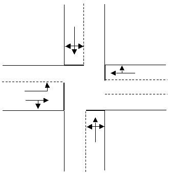
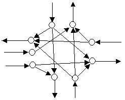
When a road network is represented as an abstract graph such as for static assignment modeling. There is a set of rules which must be followed to provide a realistic representation. i.e. intersections should be represented in terms of sub-graphs modeling the permissible movements and turn penalties are associated with those movements to represent the delays in the road network. The figure below shows an example of junction represented as a physical layout and as an abstracted network.

Aimsun Next provides three key classes of object to support the four stage modeling process:

• Road sections and nodes are used to describe the network.
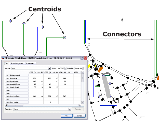
• Centroids and connectors describe the zones and link them to the road network.
• A Trip Matrix T describes the traffic demand where entries t~ij~ represent the number of trips with origin in zone i and destination zone j.

Aimsun Next provides tools to create, edit, and link these objects to form a transport model.

The figure below shows an example of OD matrix for the network of the example, in which row and column names identify the zones (centroids).

Trip Generation / Attraction Models

The first phase in the four step model is a trip generation and trip attraction process to estimate the number of trips originating and/or ending in each zone. This phase of the travel demand estimation process can be performed either at the disaggregate level of the household or at the aggregate level of the zones, when the number of trips is assumed to be a function of zonal characteristics. In what follows we will restrict our description to the aggregated models.

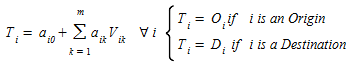
Each origin zone will have a capacity for trip generation that can be modeled in terms of its socioeconomic characteristics (land use, income level, house holding, car ownership, employment, etc.) as a function:

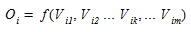(1.1)

where O~i~ is the number of trips generated by the i-th zone and V~ik~ is the k-th socioeconomic variable of the zone.

Similarly, as a destination, each zone, at the aggregate level, will have a capacity for trip attraction than can also be modeled as function of its socioeconomic characteristics:

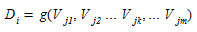(1.2)

where, as before, D~j~ is the total number of trips attracted by zone j, and v~jk~ is the k-th socioeconomic variable of zone j.

At the aggregate zonal level, the most frequently used techniques for trip generation and attraction are based on multiple regression analysis, and then a common form for functions O~i~ and D~j~ might be:

(1.3)

in which the v~ik~ values are the given trip “production” or “attraction” factors, depending on the type of model, and a~ik~ values are the parameters whose numerical values will be estimated by multiple regression after the available data from surveys, census databases and other sources. The factors of trip generation / attraction in this approach can be zones and traveler attributes, as well as other attributes as those of travel modes, travel routes, number of bus stops, or travel times and costs.

Trip Distribution Models and Algorithms

Trip distribution is the next step in the Four Step Methodology and is performed after the trip generation/attraction is completed. It consists of distributing across various destinations each of the trip origins Oi. Once the set of centroids is defined, the desired movements over the road network can be expressed in terms of an “origin-destination” matrix, whose entries specify the flow (number of trips over the time period of the study) between every origin centroid and every destination centroid in the network:

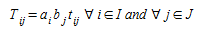
OD Matrix: T=[t~ij~]t~ij~ = number of trips between origin i and destination j

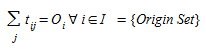
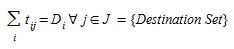
Taking into account the trip generation/attraction of each zone, the mobility matrix, also called trip matrix and Origin-Destination, OD matrix, that models the transportation demand in the area object of study, the distribution problem (Erlander and Stewart, 1990) deals with determining a non-negative matrix {t~ij:} satisfying the marginal constraints:

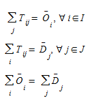
(EQN TD1)

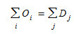
and other conditions such as the sum of departing trips is the same as the sum of arrivals:

(2.2)

Equation (2.1) means that the sum of the trips generated at each origin over all the destinations must be equal to the trip generation capacity of each origin, and the sum of all trips arriving to each destination from all origins must be equal to the trip attraction capacity of each destination.

Three methods of undertaking the trip distribution calculations are available, one by factoring growth in origin and destination matrices using Furnessing techniques, and two in Demand Modeling using a Gravity Model or a Destination Choice Model.

Growth Factor Methods (Furnessing)

Assuming that a basic or reference trip matrix {t~ij~} from a previous study or recent survey is available. The goal is to estimate a trip matrix {T~ij~} for a design year using available information about the growth rate for the study area between the year of the reference matrix and the design year.

In this case, information is available on the future number of trips originating and terminating in each zone. Therefore two sets of growth factors are available for trips in and out of each zone: a~i~ and b~j~ respectively, such that:

(2.3)

A model known as the doubly constrained growth factor; the computation of the {T~ij~}, as defined by (2.3), satisfying the conditions:

(2.4)

This requires computation of the growth coefficients a~i~ and b~j~ which is done with the Furness balancing procedure (Furness, 1965; see also Fratar 1954, Bregman, 1967).

The Furness balancing procedure is formulated as follows:

• Step 0. Initialization Set l=0 (iteration count), and 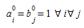(2.5)

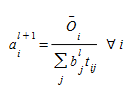
• Step 1. Balancing rows

• Step 2. Balancing columns

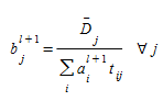
• Step 3. Stopping Test

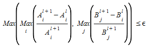
The convergence test for the process is

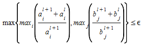
If the acceptable error ε is satisfied or l+1= lmax, (the maximum number of iterations has been reached) then STOP.

Otherwise set l:=l+1 and return to Step 1.

Ortúzar and Willumsen point out (Ortúzar and Willumsen, 1990), that growth factor methods are simple to understand and make direct use of observed trip matrices and forecasts of trip end growth. This also limits them to short-term predictions as the methods do not take into account changes in transport costs due to changes in the network. It is also important to note that they preserve the “structural zeroes”; any cell t~ij~ which equals zero in the base year OD matrix, will equal zero in the predicted T~ij~ OD matrix.

Demand Model Methods

Gravity Models belong to the family of models designed to forecast future trip patterns when significant changes in the network take place. Their name derives from the observation that volume of travel has some similarity with the force of gravity with a direct ratio to the mass (or population) of a zone and an inverse ratio to the distance between zones.

Destination choice models are a type of trip distribution or spatial interaction model which are formulated as discrete choice models, typically logit models, which assign trips through probabilities by maximizing the utility of each traveler of going from each origin to each destination. The key to this model is the assumption that the travelers select their destination based on the utility it has for them, while trying to maximize it. This model is reversible, with the same utilities, one can either use the generated trips (Departure side) or the attracted trips (Arrival side) to make the trip assignment.

Unlike the Gravity Model, the Destination Choice model does not automatically match the assigned trips to the Generation/Attraction vectors In Aimsun Next,to solve this problem, shadow prices are added to the utilities and calculated recursively. However, this is an optional part which might not be necessary and in some cases even undesirable because it distorts the utilities modeled by the user.

Comparison of Gravity Model and Destination Choice Model

A comparison between the two demand models is shown in the tables below. Note that while the Destination Choice Model offers more capability than the Gravity Model, it also requires a greater knowledge of the factors controlling demand to use it effectively. However, note that both models still omit many unobserved or unquantified attributes such as the price and quality of goods and services provided at destinations, social relationships, traveler habits, and the aesthetics of an area.

Observed Variables	Gravity Model/	Destination Choice Model
Number of Households	X	X
Number of employees by industry	X	X
Travel Time and/or distance	X	X
River crossings, highway crossings & other known psychological barriers		X
Where the traveler lives		X
Traveler's income, etc.		X
Proximity of similar, competing destinations		X
Convenience of destinations to other attractive places		X
Walkability, density, mix of uses at destinations		X
Parking Prices and Availability (sometimes)		X

Not all factors affecting choice can be directly measured. These are inferred by models.

Unobserved Variables	Gravity Model/	Destination Choice Model
Simple Random Variation	X	X
Other Traveler Attitudes / Preferences (toward price and quality of goods/services, etc.)		X
Spatial Autocorrelation / Unobserved homogeneity of destinations		X

Table derived from Travel Forecasting Resource.

Gravity Model

The general form of the gravity model is capture in the following equation:

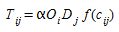(2.6)

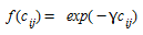
where O~i~, the number of trips generated by origin i is the “mass” of origin i, D~j~, the trip attraction capability of destination j is the “mass” of destination j, α is a constant and f(c~ij~) is a deterrence function in terms of the cost c~ij~ of traveling from origin i to destination j. The application of the formula (2.5) cannot be immediately applied as the constant cannot be determined in such a way that the marginal constraints (2.1) and (2.2) hold. This requires the introduction of additional normalizing factors A~i~ and B~j~, and the model is restated in the form:

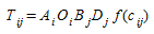(2.7)

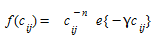
The various types of gravity models are classified by the form of the deterrence function, the most common are:

• Gravity models with exponential deterrence function
• Gravity models with power deterrence function
• Gravity models with combined deterrence function

Gravity models with an Exponential Deterrence Function

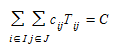
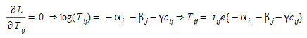
Given the undetermined nature of the model there will usually be a large number of feasible matrices for a given set of O~i~ and D~j~, because there are i*j elements and only i+j constraints in equations (2.1). This implies that a choice among the feasible matrices {T~ij~} has to be made according to some additional criterion. In order to take explicitly into account travel costs between zones when c~ij~ of the cost of traveling from zone i to zone j for all zones is available, cost can be explicitly included in the entropy model adding them as a constraint on the total expenditure in the system, when generalized costs are used, or total travel time in the system when costs are measured in terms of travel times.

The modified model is now:

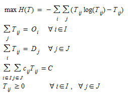(2.8)

which is again a convex optimization model whose Lagrangean function is:

(2.9)

where, as before, α~i~ and β~j~ are respectively the i-th and j-th Lagrangean multipliers of the constraint in (2.8), γ is the Lagrangean multiplier of the time constraint, and the optimality conditions hold for:

(2.10)

Then, making the changes,A~i~ O~i~=exp{-α~i~}, ∀ i ∈ I and B~j~ D~j~ = exp{-β~j~}, ∀ j ∈ J the solution can be restated as:

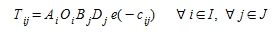(2.11)

And the balancing coefficients A~i~ and B~j~ can be calculated by the following modified Furness algorithm:

Step 0. Initialization Set l=0 (iteration count), and A~i~^0^= B~j~^0^ =1 , ∀ i , ∀ j

Step 1. Balancing rows

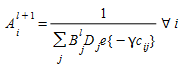
Step 2. Balancing columns

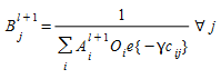
Step 3. Stopping Test

If convergence criteria less than ε or l+1= lmax, (the maximum number of iterations ) then STOP. Otherwise set l:=l+1 and return to Step 1.

A recommended estimated value for the Lagrangean multiplier γ is the inverse of the average travel cost between zones; that is γ= (average travel cost)^-1^.

Destination Choice Model

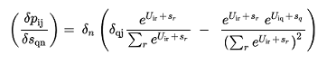
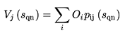
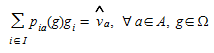
The Destination Choice Model calculates probabilities p~ij~ of assigning trips generated at origin i (O~i~) to destinations j:

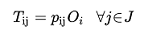(3.1)

Where i,j are the origin and destination zones and O~i~ are the generated trips by origin i.

To achieve this, a utility maximization assignment method based on a Multinomial Logit Model is used with additional (optional) functionality to match the total attraction values per destination (A~j~) calculated by the Generation/Attraction step to the assigned by the Trip Distribution Destination Choice calculation. Note that this model can also be applied in the opposite direction; using attraction values instead of generation values:

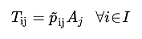(3.2)

Where A~j~ are the attracted values and p^\~^~ij~ is the probability of a traveler with destination j to depart from origin i. Because the description of this problem simply swaps origins and destinations, its description is omitted here.

Utility Maximization and Multinomial Logit Choice model

The destination choice model implemented in Aimsun Next uses a Multinomial Logit Choice model, a utility maximization model to reproduce decision-maker choices. For more detail on the model, consult https://data.princeton.edu/wws509/notes/c6s3.

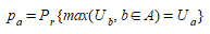
First, a utility U is a quantity which measures ”how useful is a choice for the decision-maker over another or others” - therefore choice a is preferred to choice b if:

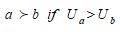(3.3)

In this case, a and b are the origin-destination pairs ij.

From Eq.(3.3) it is clear that the relative values of the utility are key; it is assumed the traveler will take the option that maximizes their utility. From this definition, the probability of choosing option a ∈ A is:

(3.4)

However, utilities are always bound to statistical errors in the attributes of the choices, which then become:

(3.5)

Where U^(0)^~a~ is the exact value of the utility and (ε~a~) is an error term.

The Multinomial Logit Model assumes that all errors are equal and have the following distribution:

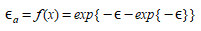(3.6)

This leads to:

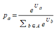(3.7)

Note that here, decisions are only based on each individual traveler's utility, which are independent of the utilities of other travelers. However, because travelers interact on the transport network, their choices are affected by the actions of others. For example, if a traveler is dissuaded by crowding or delays in option a, their decision will be affected by the number of other travelers who have taken this option.

Zero Probability Choices

In a Destination Choice Model, modifying the utilities to exclude one or more options while preserving the probabilities of the remaining options can be programmed. The process is to transform the utilities in such a way that the following statements hold:

• The probabilities of excluded choices are zero: p~a~ = 0 where a is an excluded choice (OD-pair).
• The probabilities among non-excluded choices must be invariant to maintain the order of preferences independently of other options.

(3.8)

The transformation is taken the limit of the probabilities when the utilities of the excluded choices go to ∞. This limit means that the excluded choices are never preferred over any of the non-excluded choices.

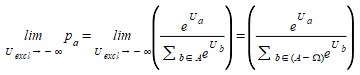(3.9)

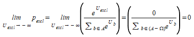(3.10)

Where a is a non-excluded choice from the non-excluded set (A-Ω) and Ω is the set of excluded options.

Numerically, this is equivalent to rescaling the denominator and setting the excluded probabilities to zero, which preserves Eq.(3.8).

Destination Choice Model with Generation/Attraction Constraints

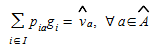
The purpose of this method is to impose the attraction constraints in the Destination Choice Model. In general, the assigned trips to each destination should match the attracted values calculated (note that, because p~ij~ are normalized, the generations match with the assigned trips by construction). Thus, in this section we describe the method to impose the following constraints:

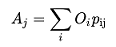(3.11)

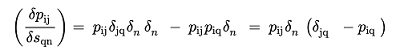
Where A~j~ is the attraction from destination j, O~i~ the generation by origin i and p~ij~ is the probability of a traveler to go from i to j which is given by:

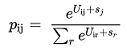(3.12)

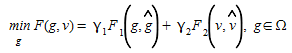
To impose all the A~j~ attraction constraints we minimize a metric that accounts for the error with the gradient descent method by modifying the utilities:

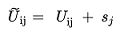
where s~j~ is their shadow pricing.

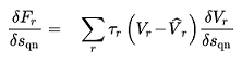
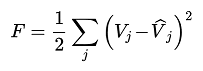
The metric is expressed as:

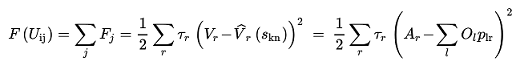(3.13)

Where τ~j~ are the (optional) weights of destination j. Note, that the function F is convex in terms of V~r~, but not necessarily in terms of s~j~.

In minimizing this metric, we impose that the attraction is equal to the total number of trips assigned to each destination as in equation (3.11).

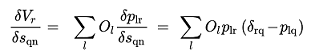
Using the gradient descent method formulae:

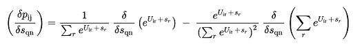(3.14)

(3.15)

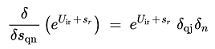
3.(16)

(3.17)

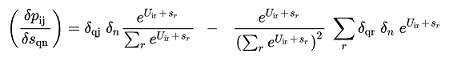
(3.18)

Therefore:

(3.19)

Can also be rewritten as:

(3.20)

And finally, the algorithm is, from step k to k+1:

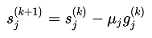(3.21)

Where μ is the (small) step size. μ might also change between steps and will be selected to minimize F.

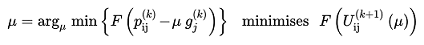(3.22)

To find the minimum:

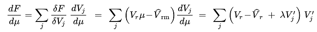(3.23)

Because s~j~ - μg~j~ is convex in μ, then, the resulting function is convex too and the stationary points are also minima and therefore global minima. To simplify the notation V~r~(0) = V~r~ and the stationary point is a minimum.

Therefore:

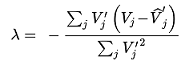(3.24)

Local Minima

There is a possibility of a multiplicity of stationary points which might be minima, maxima or a saddle. The function to be minimized can be written as:

(3.25)

It is evident that it has only one stationary point δF/δV~j~=0 , a global minimum when V^\^^~j~ = V~j~ for all j. However, in terms of the shadow prices V = V((s~q~) it is not necessarily the only minima. Therefore, to determine the stationary points (max, min or saddle):

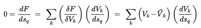(3.26)

The gradient descent method finds a local minimum by design, however there is no way to guarantee i.e. with different values of A~j~ , O~i~ and p~ij~(s~q~ = 0) that the minimum found is global. In this case, dV~k~/ds~q~ never reduces to zero and in practice:

(3.27)

Therefore using Eq.(3.9) we can find for j = q:

(3.28)

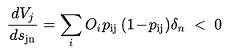
and for j ≠ q

(3.29)

The only cases when dV~k~/ds~q~ vanishes are first, when all the probabilities to go to destination j p~ij~ * are zero barring one value and second case when p~iq~ = 0. Neither of these are achieved numerically as they correspond to &s~q~ ± ∞*.

Static Traffic Assignment: User Equilibrium Models

The flow patterns through a road network can be looked upon as the result of two competing mechanisms:

• Users of the system try to travel in a way that minimizes the disutility associated with transportation.

  • Motorists driving between a given origin and a given destination are likely to choose the route with the shortest travel time.

• The disutility associated with travel is not fixed but rather depends in part on the usage of the transportation system.

  • The travel time on each of the paths connecting the origin and the destination is a function of the total traffic flow due to congestion.

Consequently it might not be obvious which of the flow patterns through the network has the shortest time. Transportation analysis looks at transportation level of service (or its inverse, travel disutility) and flows. The results of the analysis lead to a set of flows and a set of level-of-service measures that are at equilibrium with each other.

The model purpose is the description of the interaction between congestion and travel decisions that result in this flow. Because congestion increases with flow and trips are discouraged by congestion, this intersection can be modeled as a process reaching equilibrium between congestion and travel decisions.

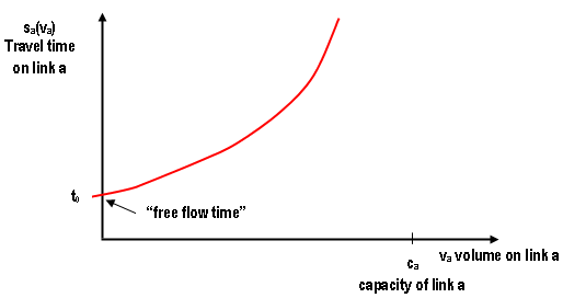
The travel impedance, or level of service, associated with the links representing a road network, can include many components, reflecting travel time, safety, cost of travel, stability of flow and others. The most common representation of this impedance is in terms of travel time, as far as empirical studies seem to indicate that it is a primary deterrent for flow and on the other hand it is easier to measure than many other possible impedance components. As has been mentioned the level of service in transportation services is usually a function of their usage. Because of congestion, travel time on road networks is an increasing function of flow. The typical representation of link impedance is in terms of the so called “volume-delay” functions, expressing the travel time s~a~(v~a~) on link a∈A as a function of the volume v~a~ on that link. These are nonlinear functions whose theoretical appearance looks as the one depicted in figure below, always under the capacity of the link.

The concept of equilibrium in transportation analysis

It is a concept borrowed from the theory of the perfectly competitive markets modeled in terms of two interactive groups: the producers and the consumers. The behavior of the producers is characterized by a supply function and the behavior of the consumers is characterized by a demand function. The supply function expresses the amount of goods that the supplier produces as a function of the price of the product. As the price increases, it becomes profitable to produce more and the quantity supplied increases.

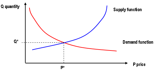
The demand function describes the aggregate behavior of consumers by relating the amount of the product consumed to its price. As the price increases, the amount consumed decreases. Figure above depicts simple demand and supply functions for a certain product. The point at which the two curves intersect is characterized by the “market clearing” price, P^∗^, and quantity produced Q^∗^. The point (P^∗^,Q^∗^) is the point at which price remains stable, this is known as the “equilibrium” point.

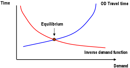
For transport systems the demand is represented in terms of a demand function that relates the number of trips to their cost (i.e. travel time) and the supply is represented in terms of a performance function (i.e. travel time between OD pairs), as in the figure below.

The user equilibrium is reached when “no traveler can improve his/her travel time by unilaterally changing routes” or, as originally formulated by Wardrop (1952), “The travel times on all the routes actually used are equal to or less than those which would be experienced by a vehicle on any unused route”, formulation known as Wardrop’s first principle or Wardrop’s User Equilibrium principle.

A simple example taken from Sheffi (1985) will help to illustrate and understand the Wardrop’s Principle. Take a simple network as the one in figure below, with only one origin and one destination connected by two alternative routes, with a total demand of q trips, generating the traffic flows x~1~ and x~2~, on routes one and two respectively, satisfying q = x~1~+x~2~.

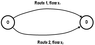
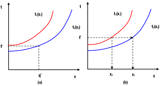
Let us also assume that travel times s~1~ and s~2~ in routes 1 and 2 respectively are determined by the performance functions s~1~(x~1~) and s~2~(x~2~) of figure below, that estimate the travel time as a function of the traffic flow on each route.

If the total flow is q < q’ , then all it is assigned to route 2, whose travel time is lower, as depicts part (a) of figure below, but for a higher flow q = x~1~+x~2~ the flow distribution in equilibrium, x~1~ and x~2~, between routes 1 and 2 has to be done in such a way that travel time s on both routes is the same, as depicted in part (b) of figure below.

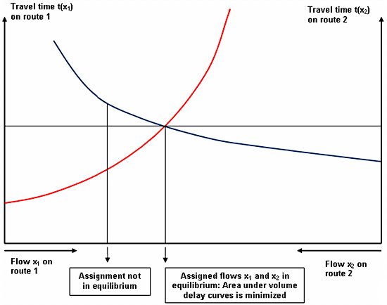
Another way to view the user equilibrium (UE), between the two routes is to superimpose the two cost (travel time or volume delay) curves (Bell and Iida,(1997) as shown in figure below. To the left of the intersection of the two curves, route 1 costs less than route 2, and there is an incentive to swap to route 1. To the right of the intersection, route 2 costs less than route 1 and there is an incentive to swap to route 2. The intersection of the two curves represents the equilibrium point at which costs of route 1 and 2 are equal and there is no incentive to swap routes. Geometrically the intersection corresponds also to the point that minimizes the total area under the cost functions; at any other point the area will be greater.

The main traffic models for the estimation of the distribution of traffic flows on a road network are based on mathematical models of route choice, that is, the modeling of how users select their routes under the prevailing traffic conditions.

The concept of equilibrium plays a central role in this model building process. Wardrop stated the two principles that formalized this concept of equilibrium, and introduced the behavioral postulate of the minimization of total costs, that along with the principles are the fundamental modeling hypothesis. Traffic equilibrium models are descriptive models that are aimed at predicting link flows and travel times that result from the way in which users choose routes from their origins to their destinations in a transportation network (Florian, 1986, and Florian and Hearn, 1995) (Sheffi, 1985).

The first principle states that "The journey times on all routes actually used are equal to or less than those which would be experienced by a single vehicle on any unused route".

The traffic flows that satisfy this principle are usually referred to as "user optimized flows", because each user chooses the route that he perceives the best. "System optimized flows" are characterized by Wardrop's second principle which states that "the total travel time is minimum".

Static Traffic Assignment Models built according to these principles and the postulate of minimization of total cost, consider a given period of time for which the demand characteristics have been determined, and estimate the flow patterns that result from the interaction of the demand and the congestion characteristics of the transport infrastructure available.

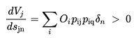
The road network is modeled in terms of a graph, whose nodes n ∈N represent origins, destinations, and intersection of links, and links, a∈A represent the transportation infrastructure, as discussed above. The flow of trips on a link a is given by v~a~, and the cost of traveling on a link is given by a user cost function s~a~(v) where v is the vector of link flows over the entire network. As these functions model the time delay for a journey on arc a, they are called volume/delay functions. A key modeling hypothesis concerning the behavior of these functions is that they are assumed to be monotone, that is such that:

(4.1)

and they are also assumed to be continuous and differentiable.

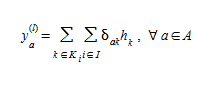
The origin to destination demands, g~i~, i ∈ , where is the set of origin/destination pairs, OD, can use directed paths k, k∈K~i~, where K~i~ is the set of paths for OD pair i. The flows on paths k, h~k~, satisfy flow conservation and non-negativity conditions:

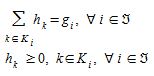(4.2)

The corresponding link flows v~a~ are given by:

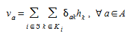(4.3)

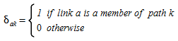
Where:

The cost of each path s~k~ is the sum of user costs of the links on path k:

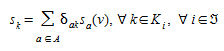(4.4)

Let u~i~ be the cost of the least cost path for any OD pairs i:

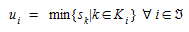(4.5)

The network user equilibrium model, based on first Wardrop’s principle, is formulated by supposing that for every OD pair Wardrop's user optimal principle is satisfied, or in other words, that all the used directed paths are of equal cost, that is:

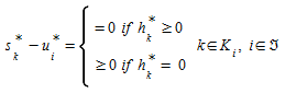(4.6)

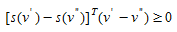
over the feasible set (4.2)-(4.3). This network equilibrium model can be restated in the form of a variational inequality:

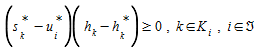(4.7)

where h~k~ is any feasible path flow. If h^∗^~k~>0 , then s^∗^~k~=u^∗^~k~ because h~k~ might be smaller than h^∗^~k~, if h^∗^~k~=0 then the inequality is satisfied when s^∗^~k~-=u^∗^~k~≥0.

By summing over k∈K~i~, and i∈, and taking into account constraints (4.2) and (4.3) when the demand g~i~ is constant, model (4.7) can be reformulated as follows (Fisk and Boyce, 1983) (Magnanti, 1984) (Dafermos, 1980):

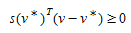(4.8)

which is the variational inequality formulation derived by (Smith, 1979).

User Equilibrium Fixed Demand Models

When the user cost functions are separable, that is, they depend only on the flow in the link s~a~(v)= s~a~(v~a~)a∈A, and demands g~i~ are considered constant, independent of travel costs, the variational inequality formulation has the following equivalent convex optimization problem (Patriksson, 1994; Florian and Hearn, 1995):

(4.9)

and the definitional constraint of v~a~ (4.3).

Although the traffic assignment problem is a special case of nonlinear multi-commodity network flows, and might be solved by any of the methods used for the solution of this problem, more efficient algorithms for solving this problem, based on an adaptation of the linear approximation method of Frank and Wolfe (Frank and Wolfe, 1956) have been developed in the past years (Leblanc at al., 1975) (Nguyen, 1976) (Florian, 1976). Other efficient algorithms based on the restricted simplicial approach have been developed by Hearn et al. (Lawphongpanich and Hearn, 1982) (Guélat, 1982) or on an adaptation of the parallel tangents method (PARTAN) (Florian et al., 1987).

The adaptation of the linear approximation method to solve the user equilibrium assignment problem requires only the computation of shortest paths and a one-dimensional minimization of a convex function. Starting from a feasible solution, the linear approximation method generates a feasible descent direction (Bazaraa et al, 1993; Sheffi, 1985) by solving a subproblem that is obtained by linearising the objective function. Then, an improved solution is found on the line segment between the current solution and the solution of the subproblem. For the UE with fixed demands formulated in (4.9) where cost functions are separable, the linearised approximation of the objective function at an intermediate iteration l when the current solution v^(l)^ is:

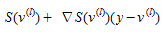(4.10)

Because S(v^(l)^) and ∇S(v^(l)^)(v^(l)^) are constants, the linearized subproblem to be solved reduces to:

(4.11)

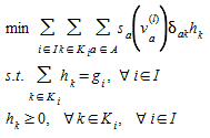
by changing the order of summation in the objective function of (4.11) and by using (4.4) the objective becomes:

(4.12)

Because the terms of the objective function (4.12) can be separated now by OD pair i, the solution of the linearized subproblem can be obtained by computing the shortest path for each OD pair i, and allocating the demand g~i~ to the links of these paths. Such a demand allocation or assignment is referred to as an “all-or-nothing” assignment. This yields the arc flow vector:

(4.13)

and the direction of descent is:

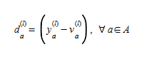(4.14)

An iteration of the linear approximation algorithm is completed by finding the solution of

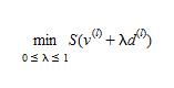(4.15)

or, equivalently, by annulling its derivative, that is, finding &lambda; where 0≥λ≥1, for which

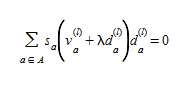(4.16)

unless the minimum of (4.14) is attained for λ=0 or λ=1.

The main computational advantage of the linear approximation method is that the paths that are used at each iteration to compute the descent direction are generated as required and need not be kept in successive iteration. This the storage requirements do not increase with the number of iterations. At each iteration only the flows v^(l)^ and the link costs s^(l)^ need to be kept, in addition to the network link data.

Because S(v) is a convex function and ∇S(v)=s(v),

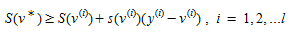(4.17)

The right hand side of (4.17) provides a lower bound on the optimal values S(v^∗^) at each iteration. The best lower bound obtained up to a current iteration l is:

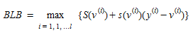(4.18)

Hence a natural stopping criterion, usually denoted as the relative gap (RGAP) is

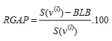(4.19)

Roughly speaking all these adaptations of the linear approximation method (LAM) lie in the following algorithmic framework (Florian, 1986; Florian and Hearn, 1995), which is the one used for the Traffic Assignment function in Aimsun Next:

STEP 1: Initialization: Find an initial feasible solution v^(1)^;s^(1)^=s(v^(1)^);l=1

STEP 2: Solution of the linearized sub-problem at iteration l

where s^(l)^~k~ is the cost on path k at iteration l. For each OD pair i the algorithm finds the shortest path k^∗^~i~ and performs an all-or-nothing assignment, finds the flows h^(l)^~k~, computes the arc flow vector y^(l)^ according to (4.12), and the descent direction d^(l)^=y^(l)^-v^(l)^ according to (4.13)

STEP 3: Verify if a predetermined stopping criterion is satisfied (i.e. RGAP≤ε). If it is satisfied, then STOP; otherwise continue to Step 4.

STEP 4: Find the optimal step size λ^(l)^ by solving (4.15)

STEP 5: Update link flows and costs

Set l=l+1 and return to Step 2.

The slow convergence of the linear approximation method in the neighborhood of the optimal solution has led to investigation of variants of the method, which could improve the rate of convergence while maintaining the simplicity and computational advantages of the linear approximations.

One method of speeding up the convergence near the optimal solution is changing the descent direction as explained in (Daneva 2002). Instead of the descent direction explained in equation 4.14, the conjugate FW descent direction is used. The conjugate FW descent direction is found as:

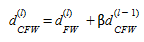(4.20)

Such that:

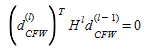(4.21)

With H^l^ the Hessian of the UE objective function in the l-th iteration.

Estimation of OD Demand Flows using Traffic Counts: Matrix Adjustment

If information is available about the current traffic flows on a subset of links of the network, with at least a significant number of links, in both number and layout, then this information can be used to adjust the local OD matrix and get a better representation of the trip patterns. In other words, we are seeking for methods aimed at improving the estimates of the current origin-destination demand flows by combining direct and/or indirect (model) estimators with other aggregated information related to OD demand flows (Cascetta, 2001). In what follows, the aggregate information will be identified with traffic counts on some links of the transportation network.

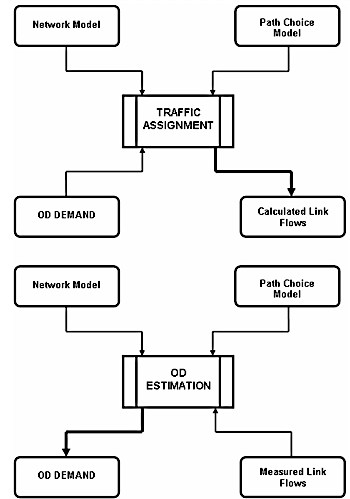
From a certain point of view, the problem of estimating OD flows by using traffic counts can be considered as the inverse of the traffic assignment problem. Traffic assignment problem can be stated as that of calculating link flows starting from OD flows, network and path choice model. Vice-versa, the problem under study is that of calculating the OD flows starting from the measured link flows, using network and path choice model (see Figure below).

Estimation of OD matrices using traffic counts has received considerable attention in recent years both from the theoretical and empirical point of view. This can be easily explained given the cost and complexity of sampling surveys, as well as the lack of precision related to both direct and model estimators of OD flows. On the other hand, it is not unusual to find an already existing detectors infrastructure on a network, making link flows (traffic counts) on some subset of network links cheap and easily obtainable, often automatically. Furthermore, in many transportation engineering applications, OD flow estimates are essentially aimed at predicting traffic flows derived from changes in the network and it is expected that a matrix capable of reproducing accurately enough such aggregates will give better predictions on the expected impacts of the network changes.

In the OD matrix estimation problem we are interested in finding a feasible vector (OD matrix) g∈Ω, where g={g~i~},i∀ I, consists of the demand for all OD pairs. One can assume that the assignment of the OD matrix onto the links of the network is made according to the assignment proportion matrix P={p~ia~},i∀I,a∀A where each element in the matrix is defined as the proportion of the OD demand g~i~ that uses link a. The notation P=P(g) is used to remark that, in general, these proportions depend on the demand.

When assigned to the network, the OD matrix induces a flow v={v~a~},a∀A, on the links in the network. We assume that observed flows, v^^^-{v^^^~a~}, are available for a subset of the links, a ∈A^^^⊆A, and that a reference matrix g^^^∈Ωis also available. The generic OD matrix estimation problem can now be formulated (Petersson, 2003) as:

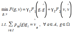(5.1)

The functions F~1~(g,g^^^) and F~2~(v,v^^^) represent generalized distance measures between the estimated OD matrix g and the given reference matrix g^^^, and between the estimated link flows v and the observed link flows v^^^, respectively.

The parameters γ1 and γ2 reflect the relative belief (or uncertainty) in the information contained in g^^^ and v^^^; and the problem can be interpreted as a two-objective problem. The two objectives are expressed in F~1~ and F~2~, and γ1 and γ2 are the corresponding weighting factors.

The set of feasible OD matrices, Ω, normally consists of the non-negative OD matrices, but it can also be restricted to those matrices within a certain deviation from the reference values, i.e.:

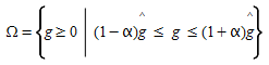
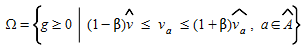
for some suitable parameter α stating the tolerance level. An analogous formulation can be used to state a maximum deviation from the link flow observation with a tolerance parameter β>0:

Another possibility is to restrict the total travel demand in all OD pairs originating or terminating at a certain node, which in the four steps model would represent an adjustment of the trip distribution with respect to the trip generation.

Obviously, the resulting OD matrix is dependent on the objective function minimized in (5.1), that is, on the choice of distance measure. One of the distances initially proposed, probably by analogy with the trip distribution problem, has been the maximum entropy function, which in its original form can be formulated as:

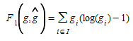(5.2)

In this extreme formulation, the reference matrix has no influence at all, and the OD matrix estimation is more a trip distribution procedure. In a more advanced entropy function, individual weights are given to each element i∈I, a case of special interest is that based on principle of minimum information (van Zuylen and Willumsen, 1980):

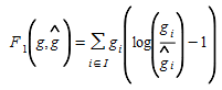(5.3)

Another type of measures are based on the maximum likelihood which maximizes the likelihood of observing the reference OD matrix and the observed traffic counts conditional on the estimated OD matrix. It is assumed that the elements of the reference OD matrix are obtained as observations of a set of random variables. For a Poisson distributed system with a sampling factor ρ the objective measure can be formulated as:

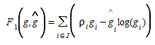(5.4)

F~2~ can be formulated in similar way as in (5.2) or (5.4).

A type of objective function which is becoming most used in these models is the one based on the least squares formulation, as for example:

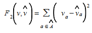(5.5)

which can be weighted using the information on the significance of each observation, as for instance when the measurements contained in v^^^ are computed as means from a set of observations for each link, then in this case we can use the variance σ^2^~a~ as a measure on how important each link observation is, and therefore reformulate (5.5) as:

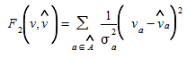(5.6)

One disadvantage of the entropy maximizing approaches as formulated in (5.1) lies in the treatment of link flow observation as constraints and therefore as error-free (Bell and Iida, 1997). A way of trying to overcome this disadvantage is using a generalized least squares approach to provide a framework for allowing for errors from various sources, the method also yields standard errors for the trip table, thereby indicating the relative robustness of the fitted values. The method was first proposed by Cascetta (Cascetta, 1984).

The equivalent optimization problem has the form:

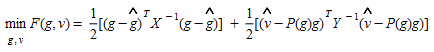(5.7)

The inputs are prior estimates of OD flows, g^^^, link flow measurements v^^^, variance-covariance matrices from the prior estimates and from the link flow measurements (X and Y respectively), and the matrix of link choice proportions P(g). As variance-covariance matrices are positive definite and the objective function is convex, the minimum is uniquely given by:

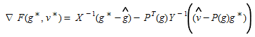(5.8)

This yields the following linear estimator:

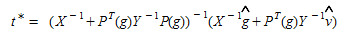(5.9)

Unlike the maximum entropy model, there is nothing to prevent negative fitted values for the OD flows being produced by the generalised least squares estimator. While negative values would reflect small real values, they are nonetheless counter-intuitive. Bell (Bell, 1991) has considered the introduction of non-negativity constraints for the fitted OD matrix.

It is well known that there are in general many OD matrices that, when they are assigned to the network, can induce equivalent link flows in the observed links. The set of constraints in the generic problem formulation (5.1) to determine g:

(5.10)

consists of one equation for every link flow observation, and thus it is an undetermined equation system as long as the number of OD pairs |I|, is greater that the number of link flow observations |A^^^|, and this especially true for large real world networks. Additionally, the information transferred through the equation system is delimited by topological dependencies. A basic principle in typical network flows is that for consistent flows the balance equations must hold or, in other words, the sum of incoming and outgoing flows at any intermediate node must be zero; a principle that can also be interpreted in physical terms by Kirchoff’s law. This means that for each intersection, at least one link flow is linearly dependent from the others, what results in a row-wise dependency for the equation system.

On the other hand the non-zero elements p~ia~(g) are non-zero because link a is part of one or more shortest paths for OD pair i∈I. However, because every subpath of a shortest path is a shortest path, every pair of nodes along a certain shortest path, is also connected through parts of this shortest path and this results in a column-wise dependency for the equation system.

Thus we can conclude that the equation system (5.10) most likely is not fully ranked, which further increases the freedom of choice for the OD estimation problem, and therefore the way of determining the p~ia~(g) becomes crucial for the quality of the OD matrix estimation model, and this is usually done in terms of how the assignment matrix P(g) is calculated, and whether it is dependent of g or not or, in other words, if the route choices are made with respect to the congestion or not.

If the assignment of the OD matrix onto the network is independent of the link flows, that is, if we have an uncongested network, P(g)=P is a constant matrix. In that case, the first set of constraints in (5.10) can then be formulated as:

(5.11)

Further, this substitution can be directly performed in the objective, i.e. in the function F~2~(v,v^^^), which reduces the OD matrix estimation to a problem in the variable g only. Assuming that the deviation measures F~1~ and F~2~ are convex, and the set of feasible OD matrices &Omega; is linear, or at least convex, the OD estimation problem can be easily solved with some suitable standard algorithm for nonlinear programming, this is the usual approach taken in most cases (van Zuylen and Willumsen, 1980).

The assumption that the assignment, i.e. the route choice, is independent of the load on the links, can be assumed realistic only in a network with a very low congestion rate, or in networks, where in the practice only one route can be used.

If we assume that the network is congested, and that the routes are chosen with respect to the current travel times, the route proportions are dependent of the current traffic situation, which in turn is dependent of the OD matrix. Thus, the relationship between the route proportions P and the OD matrix g can only be implicitly defined. The set of feasible solutions to the estimation problem (5.1), is defined as all the points (g,v) where v is the link flow solution satisfying an assignment of the corresponding demand g, then the generic OD matrix estimation problem (5.1), can be reformulated as a bi-level optimization program in the following way:

(5.12)

in which we want to find the g that minimizes F(g,v) subject to ∈Ω, under the hypothesis that the induced link flow v satisfies the equilibrium assignment conditions obtained by solving the lower level problem:

(5.13)

The core of the heuristic implemented in Aimsun Next is an adjustment method based on a bi-level optimization method (Florian and Chen, 1995; Codina and Barceló, 2004). The algorithm can be viewed as calculating a sequence of OD matrices that consecutively reduce the least squares error between traffic counts coming from detectors and traffic flows obtained by a traffic assignment. The estimation of the OD matrix requires information about the routes used by the trips contained in the OD matrix (d~ij~). It requires the definition of the route and the trip proportions relative to the total trips d~ij~ used on each route originating at zone i and ending at zone j. This information is difficult to handle and store in traffic databases, taking into account that the number of routes connecting all Origin-Destination pairs on a connected network can grow exponentially with the size of the network. This is the reason a mathematical programming approach based on a traffic assignment algorithm is used, which is solved at each iteration without requiring the explicit route definition.

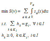
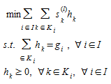
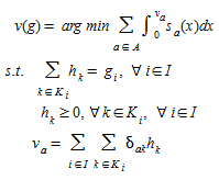
The Spiess (Spiess, 1990) bi-level optimization adjustment procedure solves the following bi-level nonlinear optimization problem:

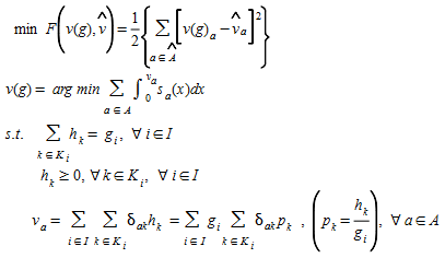(5.14)

where v~a~(g) is the flow on link a estimated by the lower level traffic assignment problem with the adjusted trip matrix g, h~k~ is the flow on the k-th path for the i-th O-D pair, and v^^^~a~ is the measured flow on link a. I is the set of all Origin-Destination pairs in the network, and K~i~ is the set of paths connecting the i-th O-D pair. s~a~(v~a~) is the volume-delay function for link a∈A. The algorithm used to solve the problem is heuristic in nature, of steepest descent type, and does not guarantee that a global optimum to the formulated problem will be found. The iterative process is as follows:

At iteration k:

• Given a s~o~ solution g^k^~i~, an equilibrium assignment is solved giving link flows v^k^~a~, and proportions {p^k^~ia~} satisfying the relationship

  

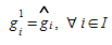
• The reference matrix is used in the first iteration (i.e.)

  

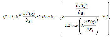
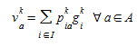
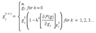
• The gradient of the objective function F(v(g)) is computed based on the relative change in the demand such that a change in the demand is proportional to the demand in the initial matrix and zeroes will be preserved in the process. This is written as:

  

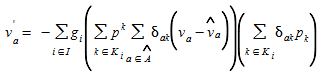
• The gradient is approximated by:

  

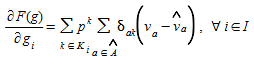
where A^^^⊂A is the subset of links with flow counts and p~k~=h~k~/g~i~.

The step length is approximated as:

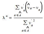
where

To ensure the convergence the step length must satisfy the condition:

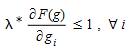
If the condition is violated for some i then the step length must be bounded accordingly: