Vehicle Exports
You can export vehicle-position data in several different formats for different reasons and uses. Aimsun Next has exporters for the following formats and purposes:
-
FZP – A format used in generating 3D-position information for importing into 3D rendering tools.
-
Versit – A local vehicle emissions model. See Aimsun Next & Versit for more details.
-
SSAM – The Surrogate Safety Assessment Model, developed with the Federal Highway Administration (FHWA) of the United States Department of Transportation. See the FHWA website for more details.
-
Discharge rate evaluation – Used to calculate saturation flows at signalized intersections.
Generating an FZP File
Information about the vehicles generated in a microscopic simulation can be exported to external packages. The purpose is to store vehicle locations in a file during a microscopic simulation. This file can then be imported into Autodesk 3ds Max® and Civil View® so that vehicles can be animated within a high-quality 3D scene. It is only available for microscopic simulations.
To export vehicle data in an FZP file:
-
Open the scenario dialog and click on the Aimsun Next APIs tab.
-
Tick the FZP Exporter option.

-
Double-click on 'FZP Exporter' to open the FZP Exporter Extension dialog. T

-
You can leave the settings as they are or you can select a new location (and name) for the output file vehicles.fzp and change the Start Time and Duration. These last two parameters specify when, in the simulation, the vehicle positions are exported.
-
Run the simulation. When the microscopic simulation finishes, the FZP file will be saved to the specified folder and will contain information about all the vehicles in the specified simulation interval.
FZP File Format
The generated FZP file consists of two parts: the header and the data. The data is organized as a semicolon-separated table.
The parameters exported to the file are:
VehNr: Vehicle ID
LVeh: ID of the next vehicle downstream
Type: Vehicle Type ID
VehTypeName: Vehicle Type Name
Length: Length [m]
t: Simulation Time [s]
a: Acceleration [m/s^2] during the simulation step
v: Speed [m/s] at the end of the simulation step
DesLn: Desired Lane (by Direction decision)
Grad: Gradient [%] of the current link
WorldX: World coordinate x (vehicle front end at the end of the simulation step)
WorldY: World coordinate y (vehicle front end at the end of the simulation step)
WorldZ: World coordinate z (vehicle front end at the end of the simulation step)
RWorldX: World coordinate x (vehicle rear end at the end of the time step)
RWorldY: World coordinate y (vehicle rear end at the end of the time step)
RWorldZ: World coordinate z (vehicle rear end at the end of the time step)
x: Distance from the start position (of the current section or turn the vehicle is in) to the front part of the vehicle, in meters, at the end of the simulation step
y: Lateral position relative to middle of the lane (0.5) at the end of the simulation step
Exporting to 3D Max Design® and Civil View®
You can import the generated FZP file into 3D Max Design® and Civil View®. Note that Civil View® enables you to assign each vehicle type to a different 3D model, but it will not perform any scaling in the object to match the simulated vehicle length.
In order to avoid unwanted overlaps and positional mismatches in the 3D scene, careful selection of vehicle types in the model is required. All vehicle types must be defined with no deviation to their length and the length should also match that of the 3D model used for visual representation in Civil View®.
For instance, in the Vehicle Type dialog below, The Length of the vehicle is fixed to 4.30 m with no variation (0.00 m in the Deviation column).

By following this general rule with all vehicle types, and assigning the correct 3D model in Civil View®, the rendered 3D scene will match perfectly with the Aimsun Next simulation.

Generating a Versit File
Versit is an emission model developed by TNO in The Netherlands (see Versit for more information). It is used to predict representative emission factors and energy-use factors for vehicle fleets where the emission factors are differentiated for various vehicle types and traffic situations. It also takes real-world driving conditions into account.
Versit uses the FZP Format for its input files but, when you are exporting data to be used in Versit, you must set the simulation step to 0.25 seconds.
Surrogate Safety Assessment Model
This section describes how the Surrogate Safety Assessment Model plug-in is used.
Note on licenses: To use this plug-in during a microscopic simulation, you need an Aimsun Next API license.
The Surrogate Safety Assessment model is a simulation and analysis project from the FHWA, which predicts the safety of roadways before accidents occur.
Documentation about the SSAM file format specification V1.04 is available from the FHWA (https://www.fhwa.dot.gov/publications/research/safety/08049).
Creating a Trajectory File
A trajectory file contains the necessary vehicle data for use in an SSAM. Only data from a microsimulation is compatible.
To create a trajectory file:
-
Open the scenario dialog and click on the Aimsun Next APIs tab.
-
Tick the SSAM option.
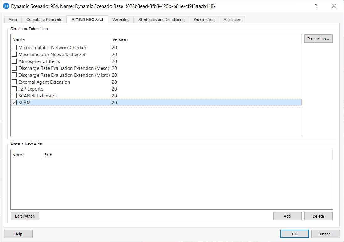
-
Double-click on 'SSAM' to open the SSAM Extension dialog.
-
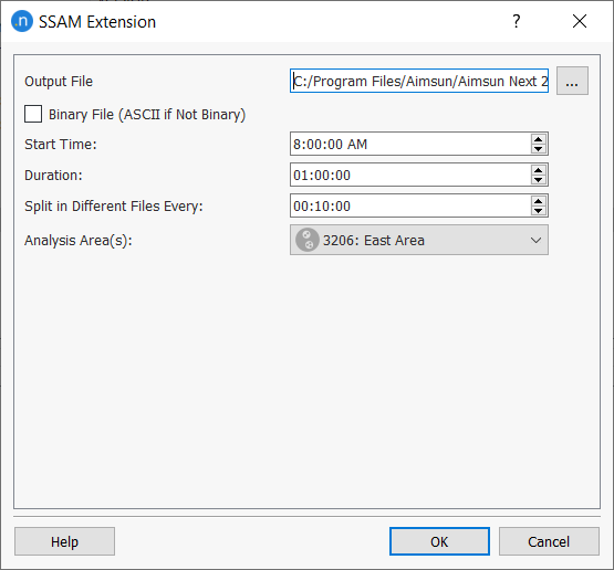
You can leave the settings as they are or you can select a new location (and name) for the output file odroutes.trj and change the Start Time and Duration. These last two parameters specify when, in the simulation, the vehicle positions are exported.
-
Optional: For Split in Different Files Every, enter a time interval. This will split the output into different files according to this interval. Files will be generated with suffixes denoting the initial time of each file.
-
Optional: For Analysis Area(s), select a grouping from the drop-down list, if available.
If the selected grouping contains sections, trajectories of vehicles are included for those in any included sections and connected nodes. If the selected grouping contains nodes, trajectories of vehicles are included for those in nodes and any sections that enter or exit any of the nodes in the grouping. Trajectory files will be split by the included groups.
-
Click OK to save the SSAM settings.
-
Click OK to close the scenario
-
Run the simulation.
Discharge Rate Evaluation
This section describes how to export a file containing vehicle headways at signalized intersections. The headways can then be used to evaluate the saturation flow of a turn. Saturation flow rate has been defined thus:
Assume that an intersection’s approach signal were to stay green for an entire hour, and the traffic was as dense as could reasonably be expected. The number of vehicles that would pass through the intersection during that hour is the saturation flow rate (Saturation Flow Rate and Capacity, University of Idaho).
To generate a vehicle headway file:
-
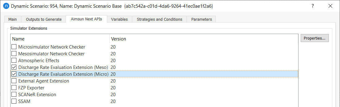
Open the scenario dialog and click on the Aimsun Next APIs tab.
-
Tick the Discharge Rate Evaluation Extension option.
Note: There are two extensions – one that works in mesoscopic simulations and one that works in microscopic simulations. Select the relevant option. If you are running a hybrid simulation, tick both.
-
Click OK.
-
Run the simulation to generate the necessary files.
File format
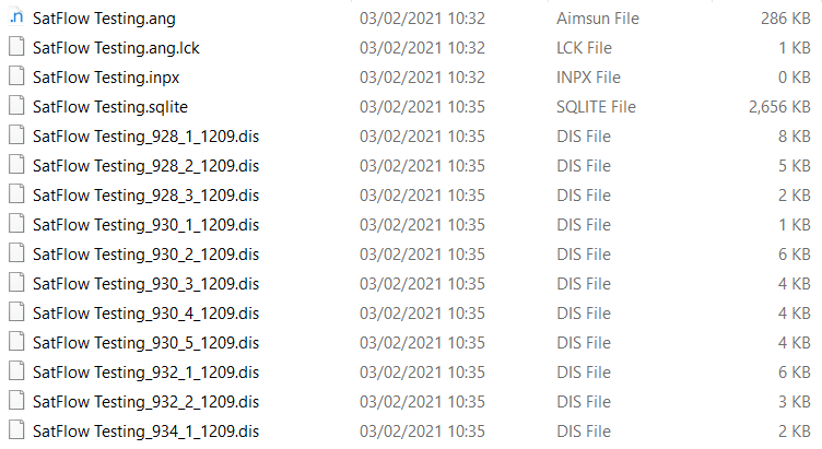
Once the simulation (or simulations) have finished, the following files are generated in the same folder that contains the ANG file:
-
A DIS file for each section lane of the signalized intersections
-
An empty INPX file with the same name as the ANG file.
-
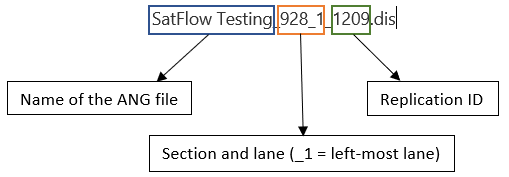
DIS file names follow this structure:
The following is an example of the content of a DIS file. The ellipsis (...) indicates that some lines have been removed due to length.
Discharge record
File: dre
Comment: Aimsun Next mini
Date: 2017-12-20T15:08:17
Aimsun Next 8.2.2[53072] Seed = 7438
Discharge at Section 330, lane index 2, signal phase 0
   90   2.39   2.55  11.40   (2: 6.97)
  180   1.00   2.58   1.99   5.21   4.28   5.34   (5: 3.88)
  270   1.15   2.37   2.07   2.22   1.65   2.40   1.83   5.64   (7: 2.60)
  360   2.44   2.39   1.98   2.26   2.09   1.74   1.91   7.88   (7: 2.89)
  450   1.85   2.51  13.94   1.79   1.75   (4: 5.00)
    ...
 3690   1.13   2.29   2.37   (2: 2.33)
 3780   2.39   2.72   1.99   2.08   3.80   2.21   4.02   (6: 2.81)
 3870   1.09   2.37   1.97   (2: 2.17)   21.23
-----      1      2      3      4      5      6      7      8      9     10
-----   2.33   3.09   3.45   3.75   3.36   3.26   3.50   4.00   2.16   2.16
-----     43     41     35     27     23     14     10      7      5      2
[164: 3.35]
-
Each line represents one signal green phase, with the corresponding headways.
-
Values after parentheses represent discharge rates of vehicles crossing the stop line of a signal after the green time (during amber or even red; there is one example, 21.23, above).
-
The 4th line from the bottom lists the index of the vehicle’s position in the queue for each signal cycle.
-
The 3rd line from the bottom contains average discharge rates for the corresponding vehicle position.
-
The penultimate line contains the number of all vehicles measured for that position (higher indices might have smaller numbers if the flow is not saturated at all times).
-
The last line lists the total number of vehicles and total discharge rate for the evaluation period.
The data can be used to calculate the saturation flow for a junction using algorithms referenced in the Transport for London Model Audit Processes 2017.