Dynamic OD Adjustment Algorithms
When flow and turn counts are available in sufficient detail and on a subset of road sections that covers most of the road network and the paths through that network, then this data can be used to refine the existing OD matrices to obtain a more accurate representation of the trips made in the network.
The dynamic OD adjustment process refines a set of existing prior OD matrices as a part of the model calibration process where the OD matrices have been disaggregated by time as well as by user class so that there are a set of matrices for time slices in the modeled period. Typically a modeled period is measured in hours and the time slices are 10 - 15 minutes in duration matching the time granularity of the observed data from roadside turn and flow counts or from loop detectors in the road. The OD Adjustment process uses a dynamic assignment to simulate the counts and flows at the detector and observation locations and iteratively refines the OD matrices one time slice with a rolling horizon.
The dynamic simulation provides
- Time dependent flows and counts as a result of assigning the current matrices to the road network in the time slice under consideration where the initial conditions in the time slice are set by the matrices assigned in previous time slices.
- The congested state of the network in each time slice
- The virtual queues of vehicles waiting to enter the network.
Adjustment Algorithm
The Dynamic OD Adjustment is formulated as an optimization problem, where the objective function to be minimized includes two parts. The first part measures the distance between the OD matrix to be adjusted and the reference OD matrix. The second part measures the distance between the observed link flows and those assigned by the model when the adjusted OD demand flows are assigned to the network.
The Spiess (Spiess, 1990) bi-level optimization adjustment procedure, which is used in the Static OD adjustment, is extended for dynamic traffic assignment (Ros-Roca et al., 2020) by including the time intervals to the problem formulation as follows:
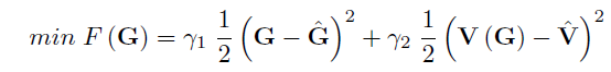
s.t. \(\textbf{G} \geq {0}\)
Where,
\(\boldsymbol{G} = \{g_{i,r}\}\) is the demand for travel for each OD pair \({i\epsilon{I}}\) in each departure time interval \({r\epsilon{R}}\). I and R are the number of OD pairs in the network and departure time intervals, respectively. \({{A'}\epsilon{A}}\), where {A} is the total number of links in the network.
\(\boldsymbol\hat{G} = \{\hat{g}_{i,r}\}\) is the reference OD matrix.
\(\boldsymbol\hat{V}=\{\hat{v}_{a,t}\}\) are traffic counts on a subset of links \(a\epsilon{A'}\) in the network equipped with detectors during time interval \({t\epsilon{T}}\). It is assumed that {T} and {R} describe the same time horizon.
\(\boldsymbol{V}\left(\boldsymbol{G}\right)=\{{v}_{a,t}\}\) are the link flows predicted by a dynamic traffic assignment of the demand \({\boldsymbol{G}}\) to the network.
\(\gamma_{1}\) and \(\gamma_{2}\) are weighting factors reflecting the uncertainty of the information contained in \(\boldsymbol\hat{G}\) and \(\boldsymbol\hat{V}\), respectively.
\(\boldsymbol{G}\), \(\boldsymbol\hat{G}\) and \(\boldsymbol\hat{V}\) are arranged as column vectors.
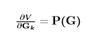
The underlying hypothesis is that \(\boldsymbol{V}\left(\boldsymbol{G}\right)\) are the link flows predicted by assigning the demand matrix G onto the network, which can be expressed as a proportion of the OD demand that passed through the count location at a certain link:
\(\boldsymbol{V}\left(\boldsymbol{G}\right) = \textbf{P}\left(\boldsymbol{G}\right)\cdot{\boldsymbol{G}}\)
where \({P}= \{p_{ir,at}\}\) is the assignment matrix. \({p_{ir,at}}\) is the fraction of the OD demand \(g_{i,r}\) for OD pair i that passes link a during measurement period t.
A gradient descent method to solve the minimization problem which follows an iterative procedure in that it calculates a negative gradient search direction and then determines the step length in this direction.
\(\boldsymbol{G_{k+1}}= \boldsymbol{G_{k}} + \boldsymbol{\lambda_{k}}*\nabla F (\boldsymbol{G_{k}})\)
\(\boldsymbol{G_{k+1}}\) is the OD matrix in iteration \({k}\). \(\boldsymbol{\lambda_{k}}\) and \(\nabla F(\boldsymbol{G_{k}})\) are the step length and search direction in iteration k, respectively.
The optimization process requires one full assignment of the OD matrices at each single iteration of the minimization procedure. The assignment matrix, \({p_{ir,at}}\) depends directly on \(\boldsymbol{G} = \{g_{i,r}\}\); so each iteration of the minimization problem requires a single dynamic assignment of \(\boldsymbol{G}\) onto the network, which is a time-consuming procedure. The computational time can be decreased significantly if we assume that \({p_{ir,at}}\) does not change significantly at each iteration, hence, a dynamic assignment at every single iteration is not needed.
As in (Spiess 1990), a Gradient Descent Method is used as the iterative procedure to solve the minimization problem, which requires one full assignment of the OD matrices at each single iteration of the minimization procedure. The assignment matrix, \({p_{ir,at}}\) depends directly on
\(\boldsymbol{G} = \{g_{i,r}\}\), so each iteration of the minimization problem requires a single dynamic assignment of \(\boldsymbol{G}\) onto the network, which is a time-consuming procedure. The computational time can be decreased significantly if we assume that \({p_{ir,at}}\) does not change significantly at each iteration, hence, a dynamic assignment at every single iteration is not needed.
The iterations are distinguished between:
Maximum Number of Iterations. Is the maximum number of iterations for the adjustment. At each iteration, the process will execute a dynamic assignment and use the path percentages obtained from it.
Gradient Descent Iterations. For each iteration of the adjustment procedure, the number of iterations of the Gradient Descent Method that will be executed without changing the path choice results, that is, without executing a new assignment.
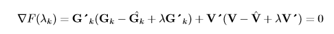
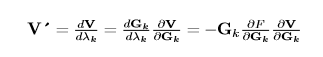
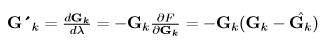
As in (Spiess 1990), the chain rule can be used to obtain the gradient of the objective function:
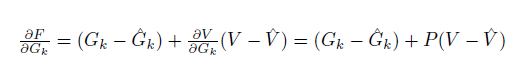
Where,
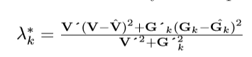
The optimal step length \(\lambda\) at each iteration k can then be calculated solving a 1-dimensional optimization sub-problem
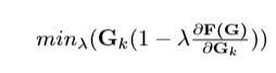
Whose solution is given by:
Where,
This leads directly to the optimal step length:
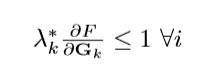
To ensure the convergence the step length must satisfy the condition:
Adjustment Process
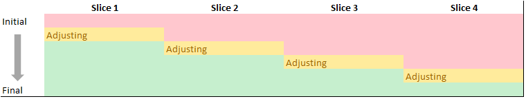
The adjustment process uses a rolling horizon where the OD matrices are adjusted starting with the first time interval and progressing to the next when the preceding one has been adjusted to match the turn and link counts. The adjustment made for each interval uses the adjustment process as used in static adjustment to update the demand for that slice using N gradient descent iterations. This ensures that for each interval the starting conditions are appropriate to that interval, based on the demand and the simulation in the preceding intervals.
The rolling horizon principle is illustrated below.
Parameters
OD Filtering
The number of OD trips to be adjusted can be large. Therefore, to reduce the number of the OD trips to be adjusted; a threshold limit can be set for OD trips to be frozen in the OD adjustment process. In order to do so the variable State Threshold needs to be defined in the Variables tab in the Dynamic OD Adjustment Scenario or Experiment.
Objective function weights
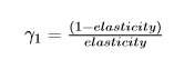
The weighting factors \(\gamma_{1}\) and \(\gamma_{2}\) in the objective function refer to the OD matrix distance and link flows distance terms of the objective function, respectively. The value(s) for \(\gamma_{2}\) correspond to the detector Reliabilities provided in the Real Data Set and \(\gamma_{1}\) is defined through the Matrix Elasticity as follows:
Ignoring Residual Paths
Residual paths are paths that only a small fraction of the vehicles use when passing through a detection point. Such residual paths can lead to strong alterations in the OD demand. The variable Proportion Threshold can be defined and a threshold value can be set to ensure that the contribution of OD pairs passing through a detection point with a fraction lower than this value will not be considered in the OD adjustment process.
Adjustment Initial Time and Duration
The Initial Time and Duration are used to specify the portion of the demand to be adjusted. There is no requirement to start at the first time slice and the Initial Time parameter in the adjustment experiment can be used to start the adjustment at a specified interval and the Duration specifies the number of intervals (after the start interval) to be adjusted. Matrices before the initial time and after the specified duration will not be adjusted and will be identical to the original matrices.