Transit Assignment

A Transit Assignment Experiment assigns the passengers in the Traffic Demand to the Transit Lines so that they can reach their destinations. The main output is the passenger loading on the Transit lines available during the Assignment period.

The Transit Assignment is based on the calculation of optimal strategies and it can take into account the capacity of Transit Vehicles.

The stages in editing and running a Transit Assignment are:

• Setup
  • Set up the transit lines with timetables.
  • Set up the transit stops with walk and waiting times.
  • Set up transit interchanges with connection times between services.
• Costs and Times
  • Set up a fare cost structure.
  • Set up the journey times.
• Transit Assignment Scenario
  • Create and run the transit scenario and experiment.

A Transit Assignment uses one of three methods to assign the passengers to the Transit Lines:

The All or Nothing Assignment calculates a single strategy or shortest path (depending on whether the option Multi-Routing is on or off) for each OD pair in an empty network and assigns the whole OD pair demand to it. Costs are updated after the assignment. Crowding Discomfort costs are not taken into account by the all or nothing calculation.

The Frank & Wolfe Assignment is based on Wardrop's first principle: for each OD Pair, all strategies or shortest paths carrying flow are of minimal generalized cost. The algorithm is based on an Optimal Strategies or Shortest Paths Algorithm (depending on whether the option Multi-Routing is on or off) and an ad-hoc implementation of a Linear Approximation Algorithm.

The MSA Assignment is a method based on Frank & Wolfe but simpler and faster because it omits one calculation – the search for the optimal step lambda – substituting this value with 1/n (n being the iteration number).

Transit Strategies

Assigning travelers to a Transit Network assumes that travelers will minimize their overall costs in the journey where cost is measured by a weighted sum of travel time in Transit Vehicles; wait times at Transit Stops; walk times to, from, and between those stops; and fare costs.

If, however, the assignment problem is regarded as simply to evaluate the path options and select the shortest path, then the problem will have been modified slightly from observed behavior. In the case of Transit, the choice of path is not selected at the outset of the journey; instead the traveler will opt to go to a particular Transit Stop and the actual path is only selected as a feasible Transit Vehicle arrives at that stop and the traveler then takes the path which is enabled by that vehicle from the set of possible paths from that location.

The initial decision is therefore a choice of strategy meaning a choice of a set of paths made from multiple sets, and the decision which particular path to take is not made at the start of the journey, but is made at some time into the journey as a bus from any of the considered lines arrives at a stop. That event then determines the actual path choice. If a journey includes two or more linked trips on Transit, then the same problem is present at the interchange; multiple sets of paths might be available, the traveler first selects a set and the choice of the second (or subsequent) part of the overall path is dependent on the arrival time of the next feasible Transit Vehicle at the interchange.

A traveler will therefore adopt a Transit Strategy (Spiess & Florian 1989) which guides the path choice but leaves the decision of exactly which path is chosen until later in the trip. A Transit Strategy has 5 steps:

1. Select a set of possible paths, starting at a particular Transit Stop, from potentially multiple available sets.
2. Go to and wait at the chosen Transit Stop.
3. Board the first vehicle that arrives which satisfies the requirements for one of the paths in the set.
4. Alight at a predetermined Transit Stop.
5. If this is the destination the trip is complete, else repeat the process with a re-evaluated strategy.

In a Static Transit Assignment, the choice of path is determined by the probability of a service being first to arrive rather than by modeling detailed passenger vehicle timings. The probability is derived from the expected wait time, assumed to be half the inter-arrival interval, at each Transit Stop. The probability that line i will be selected is in the ratio of the line frequency, divided by the combined frequency expressed as 1 / headway

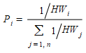
where the headway can be modified if the service is overcrowded.

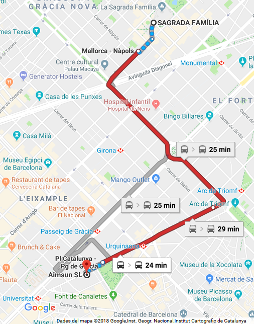
The example shown here illustrates a Transit Strategy applied to an urban journey. To go from Sagrada Família to Aimsun SLU, the traveler will calculate the options and choose a Transit Stop to start the trip. At this stop, several bus lines are available. Line 19 will bring the traveler to Arc de Triomf where transfer to lines 55 or H16 is possible, and also line 50 to Gran Vía with a transfer to line 67 will bring the traveler to the destination.

Two options are therefore available at the outset and make up the strategy but in one, the actual path will only be chosen after the strategic choice is made, and not all travelers will choose the same path, but rather there will be a certain percentage for each option available. Travelers will be split among the available options at the first stop according to the frequencies of line 19 and line 50. And for users choosing line 19, they will be then using line 55 or H16 according, again, to the frequencies of these two lines.

Transit Network

The Transit Network is composed of a set of Transit Lines with their associated costs of use, Transit Stops where passengers access the network, and Transit Stations which are groups of Transit Stops where passengers can change lines. Transit Zones structure the network by grouping stops into common cost areas.

Transit Lines

In Aimsun Next, Transit Lines are defined by a route (a set of consecutive sections), stops, and timetables. The editing details can be found in the Transit Editing section.

The assignment will calculate the frequencies of the transit lines using the specified timetables for the given assignment period.

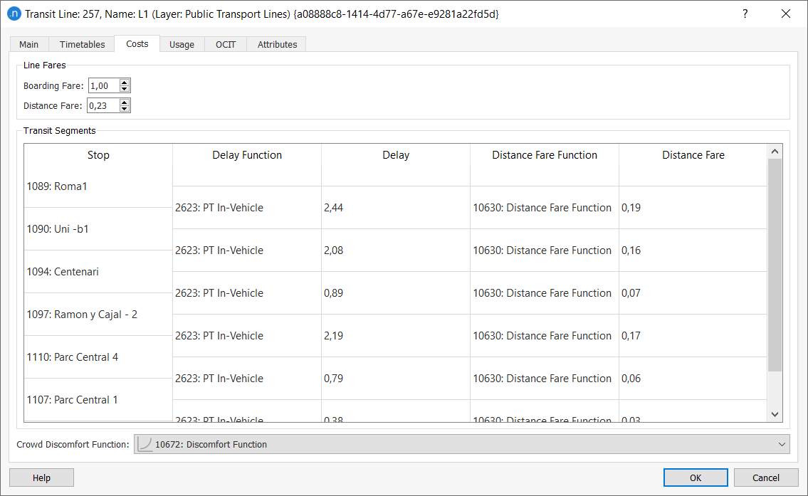
The Costs tab defines the Line Fare Constants for the line. These can be used by the Boarding Fare and Distance Fare functions, which are used to calculate fares. Delay and Distance Fare functions are selected in the Stop to Stop table or alternatively in the Transit Segments Table.

How these functions and constants are used in determining the fare costs and travel times is documented in the Transit Costs section.

The Crowding Discomfort function can also be defined here.

Circular Transit Lines

It is possible to create a circular transit line in a static transit assignment. To do so, you must ensure that the first and last section of the line are the same and contain the same transit stop at both ends. For a static transit assignment, this arrangement implies that passengers do not need to alight, board, wait, or transfer in order to stay on the transit line after the last section of the route.

Note: Dynamic simulations do not support this definition of a circular line because the transit vehicles are created at the beginning of the transit line and deleted when they reach the end of the line.

Transit Stops

Transit Stops are the start and end points of transit trips. Transfers can be made between different transit lines if a stop serves both lines.

On the Main tab, you can specify the Boarding Cost Function as described in Transit Stop Editing.

On the Static Model tab, you can specify a general Waiting Time Function, which is valid for all transit lines associated with the stop. This function can be overwritten with a specific Override Waiting Time Function for specific transit lines if required. You can also specify the walking times to and from transit stops or stations. This is described in Transit Stop Editing.

How these functions and constants are used in determining fare costs and travel times are documented in the Transit Costs section.

Transit Stations

Transit Stations group together several Transit Stops where transfers are possible between the stops. Creating Transit Stations is documented in the Transit Stations section of the Transit Stop Editor.

Connection times and walking times between stops are defined in the Connection Times and Walking Times tabs. These are documented in the Transit Stations editing section.

Transit Zones

Transit Zones group together those Transit Stops that share a specific zone cost. For example, a city might have concentric fare zones with different fare costs for trips which remain with in the central zone and trips that go into peripheral zones. Zones are created using the Transit Zones and Zone Plans editor.

Transit Costs

The cost of transit to a passenger has multiple components: a fare charged for the trip; a journey time including walk time, wait time, and travel time; and a perceived extra cost incurred as a result of discomfort and missed services due to overcrowding.

For more information about cost functions, see the Cost Functions section.

Fare Structures

The fare structure assigns a fare cost to each trip based on the policies used by a typical transport authority. These might be:

• A fixed cost for all fares.
• A fixed cost for all fares with a premium on some lines.
• A distance-related charge.
• A boarding fee plus a distance charge.

An additional fare cost can be specified when working with Transit Zones. This cost is defined in the Transit Zone Plan specified in the Transit Assignment Scenario, and it provides the additional cost for travel between different zones or within a single zone for each trip. However, this cost is allocated after the assignment, so it is not used in the Shortest Path calculation.

Aimsun Next calculates the fare as:

Fare = BoardingCost() + DistanceCost() * Distance + ZoneCost()

where the elements of the fare are calculated by the Transit Fare functions using global constants, constants defined per line, or any other algorithm you choose to code.

• Boarding Cost: This is calculated by the Boarding Cost Function. The boarding cost function is specified for every stop and its parameters are the stop and the line for which the function is called. If no function is specified, there is no boarding cost. Implementation options include:
  • A fixed rate for all lines and stops.
  • A rate fixed for a specific line at all stops. This is set in the Transit Line Editor: Costs tab.
  • A stop and line specific rate evaluated by the Boarding Function.

• Distance Cost: This is calculated using a Distance Cost Function The Distance Fare cost function is specified between stops and returns the cost between stops based on that segment distance. If no function is specified, there is no distance-related cost.

• Zone Cost: A fare cost defined in the Transit Zone Plan selected for the scenario (if any).

If required, the cost functions can use a Variable set for the scenario or for the experiment.

Flat Fare

The Flat Fare fare structure uses a single entrance fare that will be added at the first use of a Transit Vehicle and allows the passenger to subsequently transfer within the Transit Network with no additional fare cost.

When Flat Fare is enabled, Aimsun Next calculates the fare as:

Fare = Global Cost + Zone Cost

• Global Cost: An entrance fare defined in the Transit Assignment Experiment. Any passenger that uses the Transit will pay this entrance fare. Only passengers doing walk-only trips won't face this fare.
• Zone Cost: A fare cost defined in the used Transit Zone Plan (if any).

Journey Times

The journey time for a transit trip can have several components:

• The walking time from the origin centroid to the departure transit stop: This is set in the Transit Stop Editor: Static Model tab as the number of minutes taken to walk to the departure transit stop.
• The wait time at the transit stop: This is set in the Transit Stop Editor: Static Model tab, for each stop using a generic Waiting Time Function or, for each line at this stop, using a more specific override waiting time function.
• The transit delay(s) on the bus(es): These are calculated using the Transit Delay Functions between stops.
• The walk time between between transit stops when changing lines: This is set in the Transit Stop Editor: Static tab as the number of minutes taken to transfer between two stops.
• The waiting time to interchange between transit lines at a transit stop: This is set in the Transit Stations Editor.
• A penalty time for transfers specified by the Transit Transfer Penalty Functions based on the assumption that travelers will prefer a slower route with no transfers to one which includes transfers despite taking less time. The penalty function adds time to a transfer reflecting that traveler inconvenience.
• The walking time from the arrival transit stop to the destination centroid. This is set in the Transit Stop Editor: Static tab as the number of minutes taken to walk to the destination.
• For static Transit Assignments, the dwell times of transport vehicles, taking into account the aggregated volume of passengers alighting and boarding at the transit stop from the transit line for the whole assignment period. These are calculated using the Transit Dwell Time Functions.

Crowding Discomfort

Crowding Discomfort is a discomfort cost to each trip based on the discomfort generated by sharing a limited space on the Transit Vehicle. The Crowding Discomfort cost is calculated using the Crowding Discomfort Functions between stops, which are non-decreasing functions that depends on the load (volume) carried by the target Transit Line. Therefore, Crowding Discomfort cost can be used to penalize congested vehicles and force the passengers to find any other route which cost is lower.

The overall cost of the transit trip is then the monetary fare cost plus the travel time cost and crowding discomfort generated by the use of the Transit Vehicle.

Effective Frequency Congestion Model

The Effective Frequency Model can be used to simulate the failure-to-board situation that can occur in a period of heavy congestion, incrementing the waiting time cost when boarding a Transit Line that is congested. Because of that, the Shortest Path algorithm will try to find other paths with a lower cost. However, if the congested path consistently has the lowest cost, then passengers will be assigned to it. Because of that, this model cannot assure a capacity constraint and Transit Vehicles might have a load greater than their capacity.

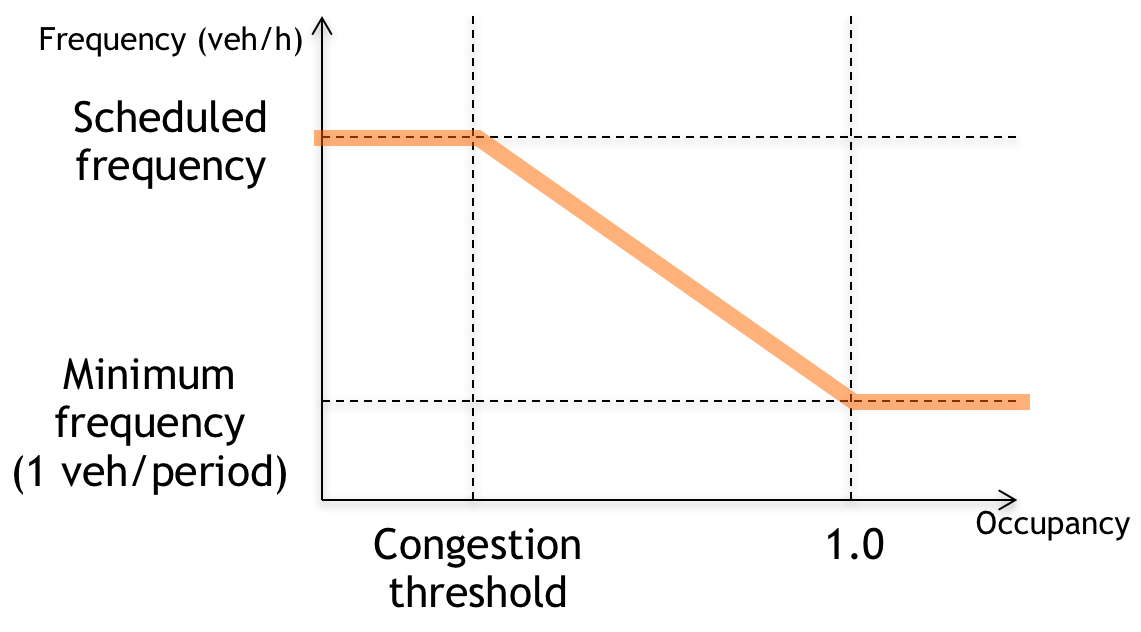
Effective Frequency Function

The effective frequency function reduces the frequency of the target Transit Line for a specific Transit Stop taking into account the residual volume (difference between nominal capacity and the volume that remains on board). More specifically, if the volume of passengers wanting to board exceeds the congestion threshold or is greater than the residual volume, the frequency is reduced linearly according to function:

Transit Assignment Scenario

To create a new transit assignment scenario, in the Project window right-click on Scenario > New > Transit Assignment Scenario.

The Transit Demand to be assigned and the Transit Plan to consider are selected as normal for a scenario. A Transit Zone Plan can also be selected to include fare costs by zone. Similarly, the time of the scenario and any relevant geometry configurations are selected. If a Real Data Set is selected, it should have Transit Loads for detectors (not sections) to validate against detection data.

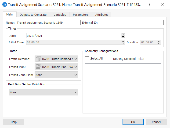
The Outputs that will be activated/stored are selected in the Outputs to Generate tab.

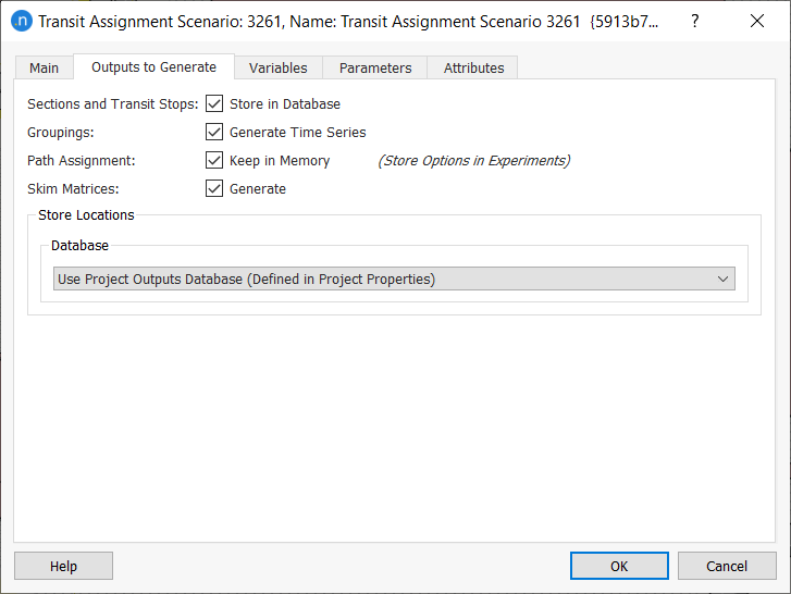
If the option to generate Skim Matrices is checked in the Scenario -> Outputs to Generate, matrices containing the costs for each component of the transit trip cost will be created under the OD matrices folder: Walking Time, Waiting Time, Fare, Transfer Penalty, In-Vehicle Time and Total Cost (combination of the previous multiplied by the user specific weights specified for the experiment). Skim Matrices will be also generated for the Function Components used in the transit trip cost functions.

Transit Assignment Experiment

An experiment is used to test different options within an Scenario. As the experiment is created, there is an option to select the assignment method.

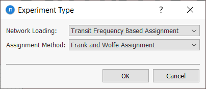
Once the experiment has been created, it can be edited by selecting Properties in its context menu or double clicking on it in the Project Window. The appearance of the experiment editor varies according to the chosen assignment method.

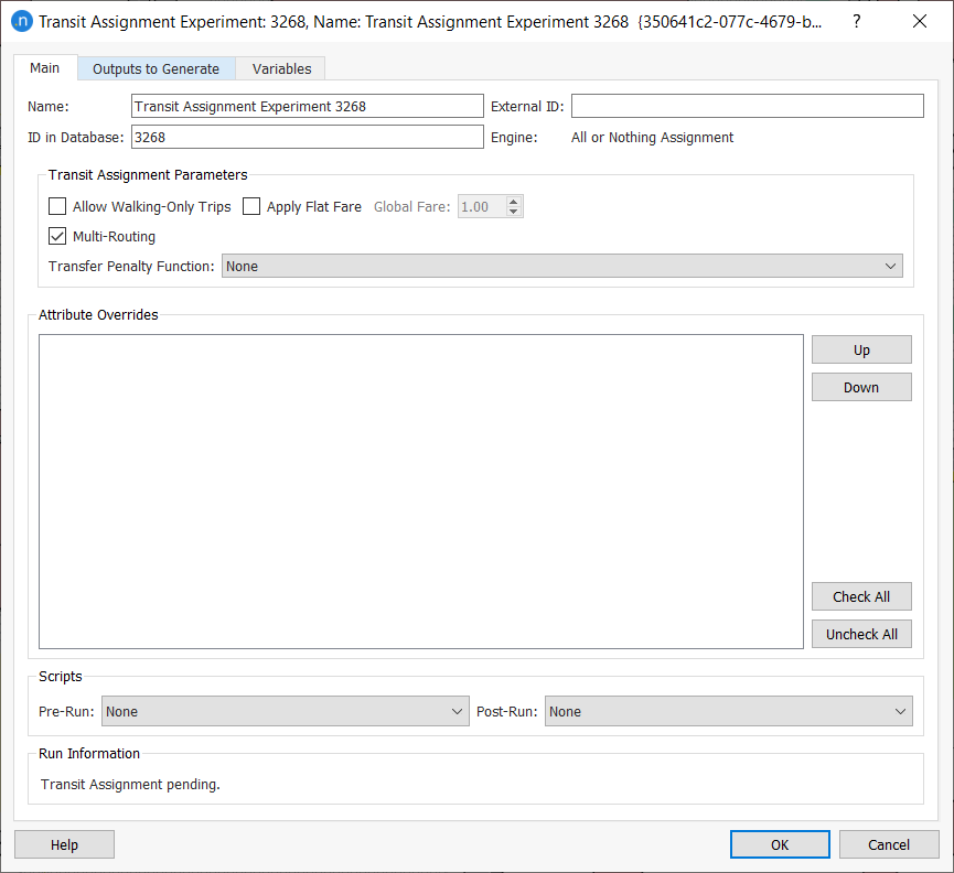
The main tab specifies the following common parameters:

• Allow Walking-Only Trips. If this option is selected, travelers can complete their trips without using Transit if both centroids are connected to the same transit stop, hence no Transit Load will be incurred by those trips.
• Multi-Routing. If this option is selected, the assignment algorithm will look for the best strategy for each OD pair. Otherwise, the assignment algorithm will only consider the best path found. When using the Multi-Routing option, it is advised that transit stops are not aggregated to a single stop: Avoid creating transit stops with a high number of transit lines stopping as this significantly increases the complexity, and hence execution time, of the route strategies calculation.

• Apply Flat Fare. Apply an entrance fare that will be added at the first use of a Transit Vehicle and do not include an additional fare if a transfer between services is required.

• Global Fare. Set the entrance fare used by the Flat Fare mode.

• Transfer Penalty Function. Transfer Penalty Function that will be applied to any transfer made in a Transit Trip.
• Dwell Time Function. This function is used to model the dwell time of transit vehicles at stops, taking into account the aggregated volume of passengers alighting and boarding at the transit stop from the transit line for the whole assignment period.
• Attribute Overrides. The overrides to be use in the Transit Assignment.
• Scripts. The pre- and post-scripts to be executed before and after the Transit Assignment.

The User costs weights for a Transit Assignment are set in the User Class Editor.

Assignment Methods

The assignment method is selected in the Transit Experiment. The methods closely follow those used in the Static Assignment Experiments for private transport.

All or Nothing Assignment

The All or Nothing Assignment has no additional parameters.

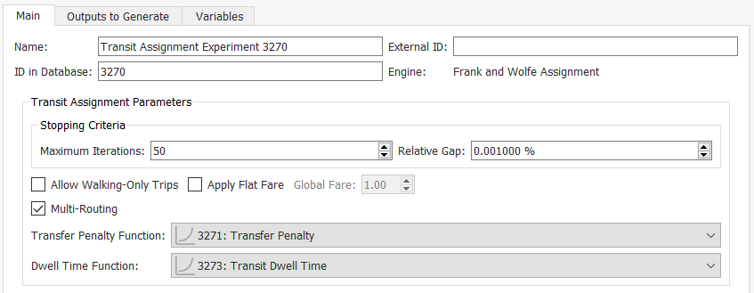
Frank & Wolfe Assignment

The Frank & Wolfe Assignment Experiment adds two extra parameters to control the iteration.

• Maximum Iterations. Maximum number of iterations to be done when executing the Transit Assignment.
• Relative Gap. Desired Relative Gap to reach and stop the execution.

It also has a parameter that enables you to select a transit dwell time function. - Dwell Time Function. This function is used to model the dwell time of transit vehicles at stops, taking into account the aggregated volume of passengers alighting and boarding at the transit stop from the transit line for the whole assignment period.

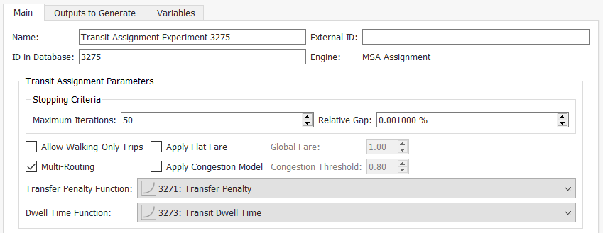
MSA Assignment

The MSA Assignment Experiment adds two extra parameters to control the iteration and two to control the assignment process.

To control iteration:

• Maximum Iterations. Maximum number of iterations to be done when executing the Transit Assignment.
• Relative Gap. Desired Relative Gap to reach and stop the execution.

To control assignment:

• Apply Congestion Model. Apply the Congestion Model to simulate the failure-to-board situation that can occur in a period of heavy congestion. This uses the Effective Frequency Model.
• Congestion Threshold. Load Factor Threshold to specify the activation of the Effective Frequency Model.

Note that the Congestion Model can only be applied in a MSA Assignment.

It also has a parameter that enables you to select a transit dwell time function.

• Dwell Time Function. This function is used to model the dwell time of transit vehicles at stops, taking into account the aggregated volume of passengers alighting and boarding at the transit stop from the transit line for the whole assignment period.

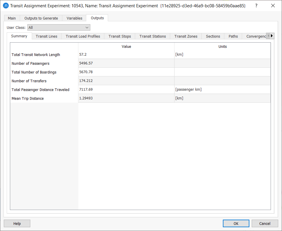
Transit Assignment Outputs

The Experiment Editor's Outputs to Generate tab holds the results for the Transit Assignment.

The Summary subtab holds the aggregated results for the entire network.

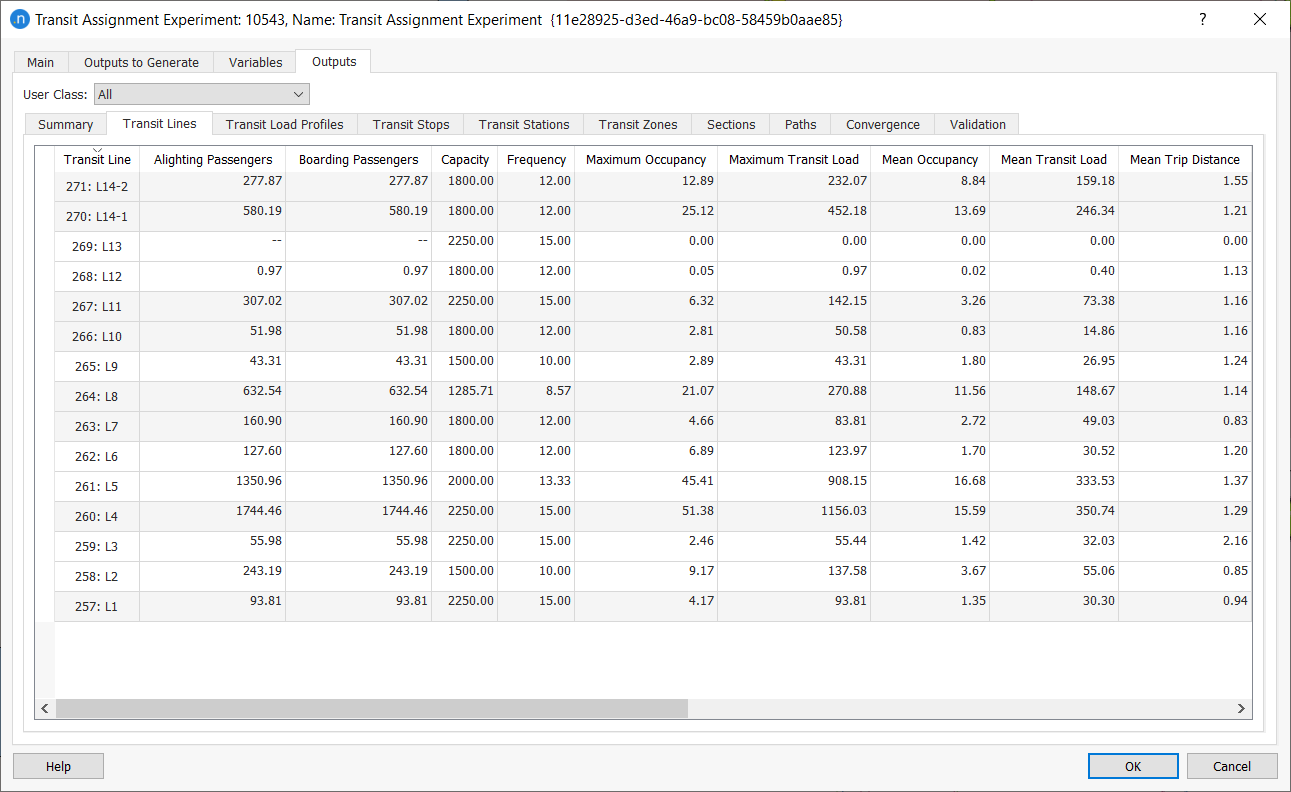
The Transit Lines subtab holds the results for each transit line. Scroll right to see more columns.

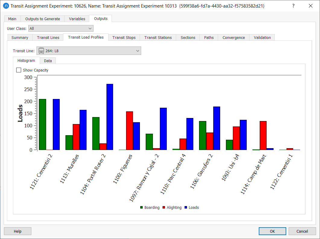
The Transit Load Profiles subtab gives a visual overview of the distribution of the load of each transit line along its route.

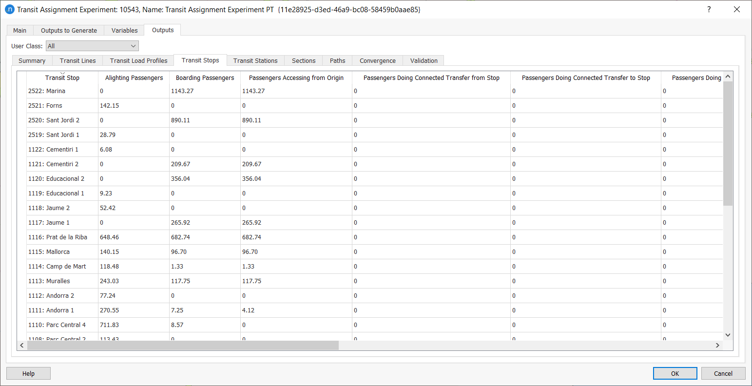
The Transit Stops and Stations subtabs hold the passenger activity at each stop, or station. Scroll right to see more columns.

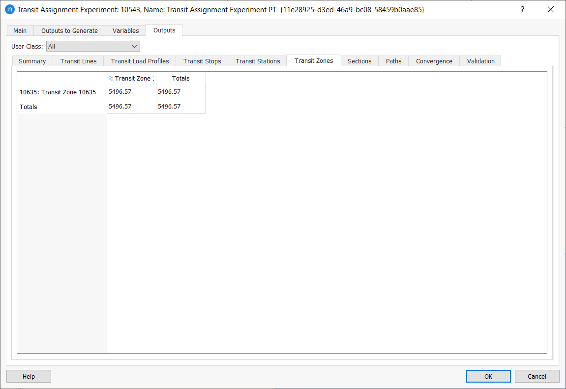
The Transit Zones subtab holds the number of trips between the Transit Zones.

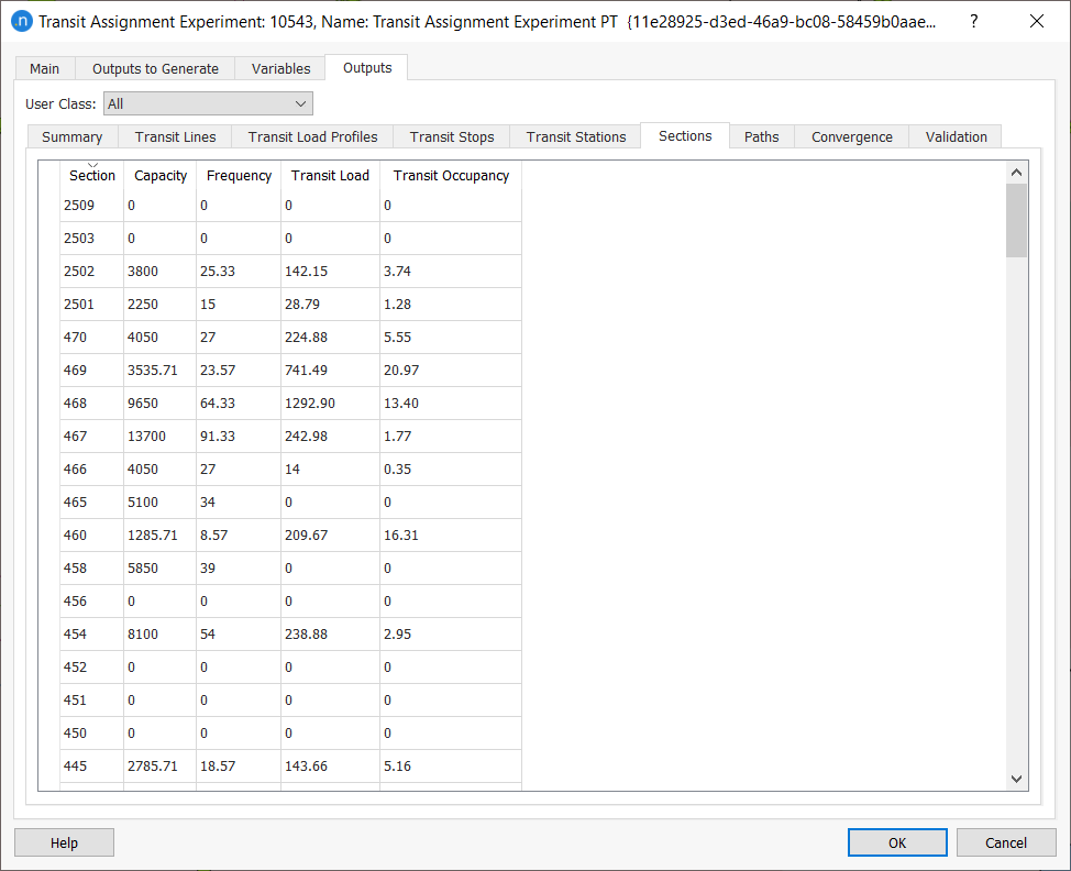
The Sections subtab holds the number of passengers traveling on each road section.

The Paths subtab is used to study which paths have been used. The results can be filtered to show only the paths selected by origin centroid, user class, destination centroid, line, or set of sections. In the paths list, the information can be expanded by clicking on a trip or path. The first level shows the aggregation of all transit assignments for each OD pair. The second level shows the aggregation of all paths for each assignment used by each OD pair. The third level shows the path information and costs. Click on the path to display it in the 2D view. Double-click on the path to open a dialog with detailed information about the path. Click the Link Analysis button to generate a visualization of the loads for the paths selected by the specified filter settings.

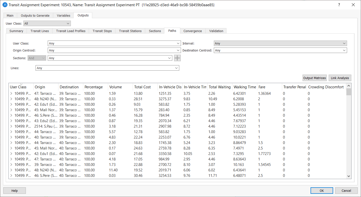
Click Output Matrices to generate the cost skim matrices for the specified filter settings in the Project > Demand Data > Costs folder.

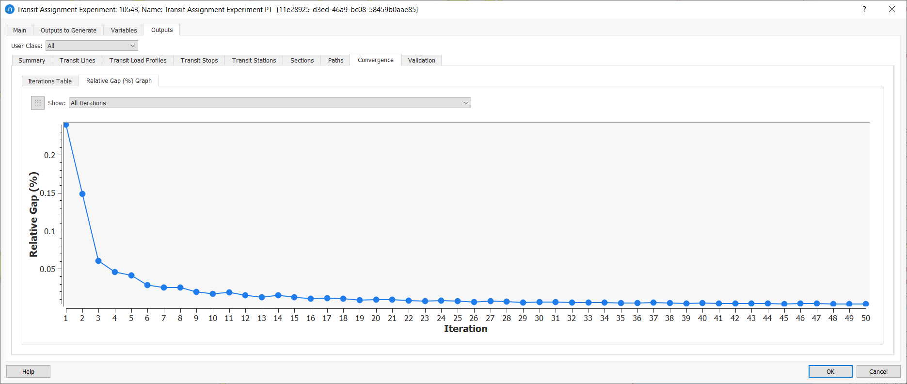
The Convergence subtab summarizes the assignment convergence in a tabular and graphical form with the option in the graph to restrict which iterations are shown.

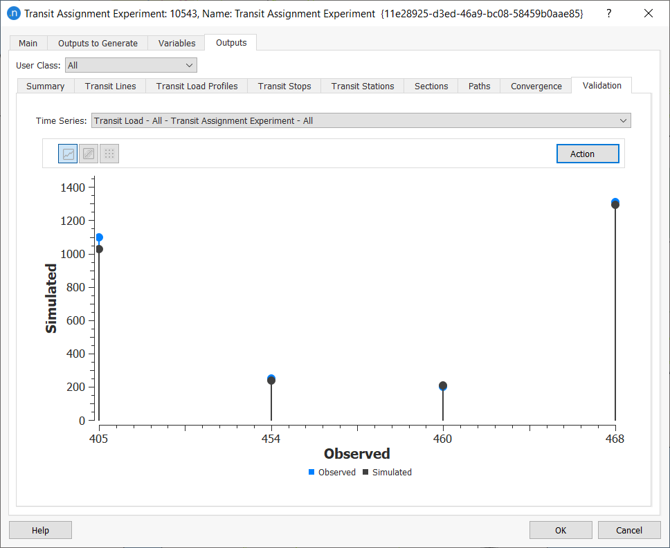
If a Real Data Set was selected in the scenario, the Validation subtab compares the assignment results against the observed data.

Associated Transit Assignment Outputs

Objects such as Detectors, Sections, Transit Stops, all contain Time Series with the transit assignment results which can be examined by clicking on the object to show its properties and selecting the Time Series tab. In the case of detectors, if there is a detector placed in a section with a transit stop, the load shown will depend on which side of the stop the detector is positioned.